- Preface
- 1 Introduction
- 2 The pillars of the Semantic Web
- 3 Web Ontology Language
- 3.1 Historical Notes
- 3.2 Ontology
- 3.3 Primitives of the OWL
- 3.3.1 An Ontology with OWL
- 3.3.2 Classes and instances
- 3.3.3 Class instances and identifiers
- 3.3.4 Class properties and literal types
- 3.3.5 Literal types
- 3.3.6 Literals facets
- 3.3.7 Relations and cardinalities
- 3.3.8 Special property restrictions
- 3.3.9 Enumerations
- 3.3.10 Generalisation
- 3.3.11 The Open World Assumption
- 3.4 Working with Protégé
- 3.5 Notable Web Ontologies
- 3.6 The Cyclists knowledge graph
- 4 Triple Stores
- 5 The SPARQL query language
- 6 GeoSPARQL
- 7 Data Transformation
- 8 Data Provision
- 9 Meta-data
- 10 Rising trends
- Annexes
- Bibliography
Copyright © 2021-2024 Luís Moreira de Sousa
This work is made available under the licence:
CC BY-NC-ND – Attribution Non-Commercial No-Derivatives
Please consult the licence document for details:
https://creativecommons.org/licenses/by-nc-nd/4.0/
DOI: 10.5281/zenodo.13892963
Version 0.3
5th of October 2024
This book is available online at:
An electronic document can be obtained from:
https://zenodo.org/record/13892963
Preface
Objectives of this book
Welcome! If you picked up this book you are possibly interested in Linked Data, on Spatial Data Infrastructures (SDI), or both. As it happens, this book encompasses the two themes, or better worded, the merger of both.
This book aims to acquaint you with state-of-the-art standards, specifications and technologies that today provide a clear path to the provision and consumption of geo-spatial data on the web. But in a semantically expressive and unequivocal way, and tapping on all referencing infrastructure offered by the World Wide Web (WWW). The path meeting the FAIR (Findable, Accessible, Interoperable and Reusable) goals to what geo-spatial data is concerned.
If you are new to the Semantic Web and Linked Data in general, this manuscript might make for a good sequential reading, especially the first introductory chapters. However, it also intends to function as a handbook, to clarify a particular doubt, to look-up on a particular method or to find a recipe setting up a necessary technology.
After reading this book you should become comfortable using ontologies, transforming data into a linked paradigm with sound semantics, querying linked data services and setting up data storage and provision infrastructures. All making use of best practices and standards issued by authoritative institutions such as the W3C and the OGC. All relying exclusively on open source software and tools.
Recent developments in data infrastructures, with novel data access paradigms based on the Open API and OData specifications, coupled with developments in the Semantic Web towards geo-spatial data are opening a new era in this domain. This book aims to be your gateway to that exciting new SDI world that now unfolds.
Intended readers
The primary target of this book are geo-spatial practitioners and scientists. The users of data services and APIs and those that set up such data access mechanisms. Data providers, be it in science, industry or public administration that wish their work to reach users according to the highest standards of quality and accessibility (e.g. FAIR).
But since this book starts by providing a general introduction to the Semantic Web and Ontology, its readership is effectively broader. The first half of this manuscript provides sufficient content for a general course on these topics, and their positioning within the wider domains of computer science and data science.
Structure
The book starts with a general overview of the motivations to adopt a Linked Data approach to geo-spatial in Chapter 1. It reviews current trends triggered by the W3C, the work of the OGC towards data access APIs and the FAIR data initiative. It goes on to pitch the Semantic Web as the vehicle fulfilling this approach.
The pillars of the Semantic Web are laid out in Chapter 2. This chapter makes you familiar with specifications such as the Unified Resource Identifier (URI), the Resource Description Framework (RDF) and the Web Ontology Language (OWL). In this chapter you can learn what are triples and the different ways of encoding them, particularly with the Turtle syntax.
Chapter 3 dives into the realm of Ontology and its application to information science. It provides the building blocks of the OWL and with a simple example guides you through the development of a web ontology from scratch. This chapter also includes instructions on different tools, both to develop and systematically document a web ontology. Finally it introduces good practices on ontology reuse, a key aspect of the Semantic Web.
The storage of RDF triples is covered in Chapter 4. Two open source technologies deserve detailed attention: Fuseki and Virtuoso. After reading this chapter you should be comfortable using both as back-end to your linked SDI.
You start to get your hands dirty in Chapter 5 with an introduction to the SPARQL query language. A collection of examples slowly makes you comfortable with the language, from obtaining simple information, to retrieving aggregates, to complex queries creating new sets of RDF triples.
With the basics of the Semantic Web introduced, the book finally delves into the geo-spatial domain in Chapter 6. The GeoSPARQL ontology is thoroughly reviewed, again with an example detailing the development of a geo-spatial web ontology. The query language aspect of GeoSPARQL is also visited in this chapter, with an exhaustive review of all geo-spatial functions defined in the standard.
In all likelihood, the data you currently work with does not exist in the form of triples, but Chapter 7 is here to help. In it you can learn various methods to transform relational and tabular data to RDF triples. Again all based on open source technologies.
With storage and transformation consolidated, it is the turn of data provision, tackled in Chapter 8. A number of methods and technologies are reviewed, with the role of the novel OGC APIs explored in more detail, particularly through the groundbreaking Prez open source server.
And since data is of no value without meta-data, the book culminates with that topic in Chapter 9. The Semantic Web is well matured in this field, offering multiple ontologies that can be combined into a rich and purposeful cataloguing of geo-spatial datasets.
Before departure there is space for a few observations in Chapter 10 on where geo-spatial Linked Data may be headed next. Emerging directions of development are briefly sketched, so you may evolve your Linked SDI in a suitable path.
Acknowledgements
I would start by acknowledging the role Jorge Mendes de Jesus had on the development of this book. It was his endearing crave for novel technologies that eventually lead me to dive seriously into the Semantic Web. Throughout the past decade his insights and experiments have constantly challenged my own understanding, definitely contributing to propel my career.
Rául Palma and Bogusz Janiak also contributed mightily to the fruition of this manuscript, even if indirectly. Working with them put me in contact with best practices in the Semantic Web, plus myriad technologies that truly enable the Linked Data paradigm. It was from the cooperation with Rául and Bogusz that I realised the need for this book.
Important was also the space created at ISRIC to pursue a Linked Data agenda. While much to the initiative of Jorge Mendes de Jesus, it were Bas Kempen and Fenny van Egmond who fostered research and experiment on this field. Their work eventually coalesced on the GloSIS web ontology and all consequent developments in soil ontology and data exchange.
Finally I thank those individuals that supported me on a personal level throughout this period. Beyond my family I would name Susana, Jeroen, Amy, Ian, Marisa, Christiane and Daphne.
1 Introduction
This chapter offers a first contact with the key aspects of Linked Data and the Semantic Web. Even if you are already familiar with both paradigms it is important to fully understand the impact they have on data exchange and use. And on the particular case of the geo-spatial data, the Semantic Web is bringing about changes that are nothing short of a revolution.
1.1 What is Linked Data?
Mostly likely, as you open this book, you already have some understanding of what Linked Data means. The term coined by Tim Berners-Lee in 2006 has become a household name, both in computer science as in data science. Even if that is the case, it is important to understand what Linked Data stands for and why it is significant. If you never heard the term before do not fear, hopefully these pages provide a simple enough introduction.
1.1.1 My data
Data. For most folk working in data science or even GIS, data equates to a flat table, possibly with field names in the first row and values in the reminder. Spreadsheets, data frames, the names are many to signify this basic and largely unstructured construct. The problems with such a frugal paradigm are many, but the concern here is the actual meaning of each datum, which goes well beyond the format.
Consider Table 1. It presents a data fragment with various columns. What exactly does it represent? There are geographic coordinates and dates and possibly some kind of measurement. Longitude and latitude are obvious terms, but to which geodetical datum do they refer? One can assume the WGS84, but on which epoch? Then there is the date, since the columns are written in English one can assume it refers to the Gregorian calendar, but some countries use a different calendar. Finally there is the Height column, beyond understanding it as a measure few other conjectures can be made. The height of what? Measured on which units?
| Lon | Lat | Date | Height |
|---|---|---|---|
| 43.1 | -19.2 | 5.0 | |
| -101.9 | -32.7 | 2010-01 | 3.2 |
Perhaps you have dealt with similar situations in the past. In fact the difficulties in identifying the true meaning of data is one of the contributing factors to the emerging informal discipline of “data wrangling”. Before feeding data to their processes, data scientists must correct errors, remove redundant and incomplete records, and consolidate datasets from different sources. Without the precise meaning of each datum and datum class, this work becomes far more complex and laborious.
A survey conducted by Crowdflower in 2016 revealed that data scientists spend up to 80% of their work time on data wrangling (Crowdflower 2016). This high figure has since been contested, but subsequent surveys have pointed to this being indeed the activity on which data scientists spend the majority of their time (Anaconda Inc. 2020). It is not statistical analysis, predictive modelling or even data representation that occupies the life of data scientists. Most of the time they are just trying to figure out what the data are and how to use them.
Essentially, Linked Data aims to address these problems. Make data easy to discover, identify and understand. If instead of simple names, the first row of Table 1 contained hyperlinks to detailed and universal definitions of those quantities the life of the data scientist would be greatly simplified. Linked Data is not so much about the links, but rather about making data unequivocally and universally understandable. Keep this simple concept in mind, the details of the how will flow throughout this book.
1.1.2 Principles
Linked Data was a concept proposed to fully express the impact of the Semantic Web on data exchange (Tim Berners-Lee 2006). Its broad idea is to present data on the web not as a set of enclosed silos, but rather as a network. It is a different paradigm to represent and exchange data. While it may appear alien, it is rather powerful and closer to how humans think and information exists in the real world. Today the principles of Linked Data can be resumed into three core ideas:
Data are primarily represented by links. Therefore every datum that is not a literal points to a resource providing further meaning or context. Record identifiers, units of measurement or concerned variables, all are represented with links leading to their precise definition and interpretation.
Data relate in networks. As every non literal is a link, data are arranged in a network. And different networks connect to each other building large constellations of data.
Data is readable by both humans and machines. Linked data form large networks of information on the internet that computer programmes may easily browse. However each link resolves to a resource (e.g. document) that is directly interpretable by humans.
The vision of data as a network of information is not at all abstract. In the real world information does not exist in silos, and has always multi-dimensional relations within itself. Humans capture information leaning it down to a convenient form. For most readers data equates to tabular records like the one in Table 1, possibly not even normalised. Linked Data is completely different, it is not laid out in tables and records, they build networks, or as they are more commonly known: Knowledge Graphs.
1.1.3 The Semantic Web
You may have already heard of the Semantic Web (SW), possibly even as a synonym of Linked Data. In fact it is an umbrella term encompassing standards and specifications issued by the World Wide Web Consortium (W3C) (Tim Berners-Lee, Hendler, and Lassila 2001). The Semantic Web is an infrastructure realising the broad vision of Linked Data, but admittedly the latter may exist without the former.
Chapter 2 reviews in the detail the main building blocks of the Semantic Web. In general terms its character can be synthesised into:
URIs embody links: links follow a determined structure, and may have different nature. They also function as unique identifiers in the World Wide Web (WWW).
Data are expressed as triples: the atomic datum element reflects human speech but is also understandable by machines.
Ontologies are expressed as triples: the same paradigm expresses both data and ontological meaning. Ergo, ontologies are machine readable.
Data sources are all linked in a federation: any data source in the Semantic Web can be combined with any other, not matter how many. Be it to reason upon the data or simply to retrieve relevant sub-sets of data.
Everything is allowed unless explicitly forbidden: data can be expressed and used in any way or form convenient to the end user (human or machine), as long as ontological restrictions are met.
While in the present day Linked Data is sometimes perceived as a broader concept, this book takes solely the Semantic Web path to geo-spatial data on the web. It will take you from the core specifications that intertwine with the WWW itself, through the theoretical foundations of ontological expression as Linked Data and then into the practical specifications making for the provision and consumption of geo-spatial data.
1.2 The Impact of the Semantic Web
1.2.1 The Five Star ranking and Linked Open Data
At the same time he proposed the concept of Linked Data, Tim Berners-Lee also put forth a five star rating system to guide data providers (Tim Berners-Lee 2006). This system thus presents a series of steps data providers must take to render their data truly web enabled, truly Linked Data (Figure 1). The Five Start Data rating system is summarised in Table 2.
| * | Available on the web (whatever format) but with an open licence, to be Open Data. |
| ** | Available as machine-readable structured data (e.g. Microsoft Excel instead of image scan of a table). |
| *** | Two stars plus non-proprietary format (e.g. CSV instead of Microsoft Excel). |
| **** | All the above plus: use open standards from the W3C (RDF and SPARQL) to identify things, so that people can point at your data. |
| ***** | All the above, plus: link your data to other people’s data to provide context. |
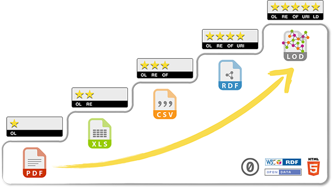
Berners-Lee went further to define the restrict result of the Five Start Data ranking as Linked Open Data (LOD). Without an open licence data may be linked, but cannot be used freely by everyone. Closed Linked Data can be relevant and useful within corporate contexts, but it is not usable by third parties. The Five Star Data ranking system eventually became synonym with LOD.
A dedicated web site has been created to help promoting the concept of Linked Open Data 1. It summarises good practices, links to training contents and provides successful examples of LOD provision.
1.2.2 Spatial Data on the Web Best Practices
In the geo-spatial domain the “game changer” would result from a joint W3C-OGC initiative embodied by the Spatial Data on the Web Working Group (SDWWG). In 2017 this work group published a report titled “Spatial Data on the Web Best Practices”, that brought into question the overall philosophy behind the OGC’s standards for digital data provision (Tandy, Brink, and Barnaghi 2017). Standards such as the Web Mapping Service (WMS), Web Feature Service (WFS) or Web Coverage Service (WCS), are all based on the Simple Object Access Protocol (SOAP). Throughout the past two decades they became the backbone of Spatial Data Infrastructures (SDI). However, SOAP is an application communication protocol whose development dates back to the 1990s, prior to the emergence of the SW. While many standards and applications came to rely upon SOAP, it is today a largely outdated protocol, that does not tap on the full potential of the internet. The main issues identified by the SDWWG with the SOAP philosophy applied to geo-spatial data can be summarised as:
- URIs are not used to identify spatial resources on the web.
- Modern API frameworks, like the OpenAPI (Miller et al. 2021), are not being used.
- Linked Data is fundamental to the provision of spatial data on the Web.
- SDIs based on OGC web services are difficult to use:
- OGC Web services do not facilitate indexing of their content by search engines.
- By design, catalogue services only provide access to meta-data, not the data themselves.
- It is not possible to access data trough links (e.g. URLs), in most cases it is necessary to construct some kind of query.
- It is often difficult for non-domain-experts to understand and use the data.
To address these issues the SDWWG proposes a five point strategy inspired on the Five Star Scheme:
| * | Linkable: use stable and discoverable global identifiers. |
| ** | Parseable: use standardised data meta-models such as CSV (Shafranovich 2005), XML(Bray et al. 2006), RDF (Schreiber and Raimond 2014), or JSON (Bray 2014). |
| *** | Understandable: use well-known or at least well-documented vocabularies/schemas. |
| **** | Linked: link to other resources whenever possible. |
| ***** | Usable: label your document with a license. |
The SDWWG then goes on to describe a series of best practices towards these five goals. Their aim is to bring geo-spatial data provided by SDIs de facto to the Web. Among those four should be highlighted:
- Best Practice 1: Use globally unique persistent HTTP URIs for Spatial Things.
- Best Practice 2: Make your spatial data indexable by search engines.
- Best Practice 3: Link resources together to create the Web of data.
- Best Practice 12: Expose spatial data through ‘convenience APIs’.
This manuscript guides you through the methods and tools empowering your SDI to do achieve exactly this.
1.3 FAIR Data
Many scientific and industrial fields transitioned from a state of data wanton to data galore during the past decade. In a short period, interpreting and using data became a major concern, as voluminous data sets pile up without use. This problem led to the assembly of a wide consortium of data stakeholders, encompassing academia, industry and government. One of the goals of this consortium was to facilitate automated access and reuse of scholarly data, but in a way that would also ease these tasks to humans. This initiative would eventually lay out what became known as the FAIR principles (Wilkinson et al. 2016).
FAIR stands for Findable, Accessible, Interoperable and Reusable. They can be regarded as a minimum set of standards without which machines and humans are incapable of using a dataset. Note that these go well beyond the concept of “Open Data”. A dataset may be open but not really usable in practice.
Soon enough the FAIR principles were adopted as goals by governments, notably by the European Commission in 2016 (Commission 2016). Still that year these principles were endorsed by the G20 (Leaders 2016). Many similar initiatives ensued, with institutions promoting FAIR principles appearing around the world. FAIR principles became a component of initiatives such as the European Open Science Cloud (Mons et al. 2017) or the European Digital Single Market (Commission 2016). The Go FAIR initiative 2 is perhaps the most visible of these efforts.
1.3.1 The Principles of FAIR
The sub-sections below go through each of the principles, as currently detailed by Go FAIR (FAIR 2022). The process towards compliance with these principles is also known as “FAIRification”.
These principles refer to three types of entities: data (or any digital object), meta-data (information about that digital object), and infrastructure. For instance, principle F4 defines that both meta-data and data are registered or indexed in a searchable resource (the infrastructure component).
1.3.1.1 Findable
The first step in (re)using data is to find them. Meta-data and data should be easy to find for both humans and computers. Machine-readable meta-data are essential for automatic discovery of datasets and services, so this is an essential component of the FAIRification process.
F1. (Meta-)data are assigned a globally unique and persistent identifier.
F2. Data are described with rich meta-data (defined by R1 below).
F3. Meta-data clearly and explicitly include the identifier of the data they describe.
F4. (Meta-)data are registered or indexed in a searchable resource.
1.3.1.2 Accessible
Once the user finds the required data, she/he needs to know how can they be accessed, possibly including authentication and authorisation.
A1. (Meta-)data are retrievable by their identifier using a standardised communications protocol
A1.1. The protocol is open, free, and universally implementable
A1.2. The protocol allows for an authentication and authorisation procedure, where necessary
A2. Meta-data are accessible, even when the data are no longer available
1.3.1.3 Interoperable
The data usually need to be integrated with other data. In addition, the data need to interoperate with applications or workflows for analysis, storage, and processing.
I1. (Meta-)data use a formal, accessible, shared, and broadly applicable language for knowledge representation.
I2. (Meta-)data use vocabularies that follow FAIR principles
I3. (Meta-)data include qualified references to other (meta)data
1.3.1.4 Reusable
The ultimate goal of FAIR is to optimise the reuse of data. To achieve this, meta-data and data should be well-described so that they can be replicated and/or combined in different settings.
R1. (Meta-)data are richly described with a plurality of accurate and relevant attributes
R1.1. (Meta-)data are released with a clear and accessible data usage license
R1.2. (Meta-)data are associated with detailed provenance
R1.3. (Meta-)data meet domain-relevant community standards
1.3.2 The role of Linked Data in FAIR
The FAIR data principles function both as an enabler and a benefactor of Linked Data. They largely overlap with the Five Star data ranking in the aims to make data usable and interconnected. There is thus a confluence of goals highlighting the impact of Linked Data. In the opposite sense, the Linked Data paradigm provides the means to achieve many of the items in the FAIRification process.
It is worth to outline the role of Linked Data in achieving all items in the Interoperable component. By design, I1 to I3 are met by specifications in the Semantic Web. And perhaps more important is R1.3, in which the FAIR data principles acknowledge the need for an ontological or semantic dimension to render data effectively reusable.
Quite how Linked Data achieves these goals is the topic for the coming chapters.
2 The pillars of the Semantic Web
The Semantic Web is an umbrella designation for a collection of specifications issued by the W3C. Starting with the Uniform Resource Identifier (URI), then with the Resource Description Framework (RDF), further with the SPARQL query language, and finally with the Web Ontology Language (OWL). These four specifications are the backbone of the Semantic Web, setting the canonical path to Linked Data.
With time the W3C came to publish many other specifications, that augment or complement the Semantic Web. Some are referred in later stages of this manuscript, others are too specific for a direct reference. But among these is GeoSPARQL, the bridge from the Semantic Web to geo-spatial data. This specification is presented thoroughly in Chapter 6.
2.1 Uniform Resource Identifier
2.1.1 Overview
At face value this section may come out as esoteric and perhaps not the most interesting subject in the context of data exchange and SDIs. Therefore, if you feel you already have a good grasp on what a URI is you might well skip it. However, the concept of a URI is fundamental to the Semantic Web, and to data sharing over the internet in general.
If you worked with a database before, or even with an unstructured dataset like a CSV file, you know the importance of identifying each data element or data record. Usually this is achieved with sequential integers, like the row number in a CSV file or an auto-increment field in a relational database. That works fine to identify data elements that exist within an isolated dataset, but when we consider sharing data over the internet that scheme simply fails.
This is a problem URIs solve: provide unequivocal identifiers that are valid everywhere and every time. They guarantee that no other data on the internet gets mistaken with your own, and that their precise meaning is unambiguous.
Beyond identifying data, URIs serve also as locators, thus performing the crucial role of networking different data and data sources. In essence they are the links in Linked Data.
A Uniform Resource Identifier (URI) is a unique sequence of characters that identifies a logical or physical resource used by digital technologies (Tim Berners-Lee 1994). URIs may be used to identify anything, including real-world objects, such as people and places, concepts, or information resources such as web pages and books.
The URI specification is meant to be hierarchical, it can be further specialised for increasingly bespoke purposes. This section covers two specialisations that are most relevant in the Semantic Web: the URL and the URN. They are primarily used to locate resources on the internet, however, a URL can also locate resources in a file system or in a closed, private network.
2.1.2 Specification
In its most basic form a URI is formed by two character sequences
separated by a colon character (:):
scheme:path (T.
Berners-Lee et al. 1998). The scheme is a string that identifies
a particular protocol used to retrieve the resource. The Hyper Text
Transfer Protocol (HTTP) is the most used, but many others exist (Klyne 2023). In
abstract, it is possible to use any scheme, even an ad hoc one.
The path determines the specific location of the resource using the
scheme declared. The most simple form of organising a path is using the
forward slash character (/) to specify a path through a
hierarchy, similar to the folder structure in a file system (a few
examples in Listing 1).
Listing 1: Abstract URI examples
scheme:path/to/some/resource

scheme:country/state/county/city
The path can also start with the identification of a host, usually a
network node that makes resources available according to the specified
scheme. In certain schemes, like HTTP, host names are managed and
assigned by an authority. When the URI includes a host name, the path
must begin with a double forward slash (//). A good example
of an authority is the W3C itself, that manages hosts identified by the
string www. Listing 2 shows a URI identifying an hyper-text
document published at the W3C’s website.
Listing 2: URI linking to a HTML document published by the W3C through the HTTP protocol.
https://www.w3.org/Addressing/URL/uri-spec.htmlThe authority assigns the host name to an institution, usually the
host name reflects the name of the institution itself. The institution
is thus responsible for the structuring of the host name into sub-names
(e.g. inspire.ec.europa.eu). In the Semantic Web the host
name in a URI further expresses responsibility for the resource it links
to (e.g. data, semantics).
A further relevant component to the path is the identification of a
fragment, i.e. a particular element or section within a resource. The
fragment is another character string positioned at the end of the URI,
separated from the path with a hash character (#):
scheme://host/path#fragment. A good example is the
identification of a heading within an hyper-text document (Listing
3).
Listing 3: URI linking to the fragment of a HTML document.
https://www.w3.org/Addressing/URL/uri-spec.html#Examples A URI can get considerably more elaborate with the query segment. It
features between the path and the fragment, and is optional as the
latter. The question mark character (?) sets its beginning,
and is then composed by a series of key-value pairs. Each pair is
separated by an ampersand (&) or a semi-colon
(;) , with the pair itself separated by an equal character
(=). Listing 4 shows an example with two key-value pairs.
There is no theoretical limit to the number of pairs the query segment
may include, resulting in long URIs. While it may come across as
cumbersome, the query segment is an important element in passing
information to remote services or applications. The query segment is
rarely employed in the context of the Semantic Web, but it is important
to be aware of its role.
Listing 4: URI including a query segment.
https://www.w3.org/Addressing/URL/uri-spec.html?key1=value1&key2=value2 This was just a brief introduction to the URI specification, it goes far beyond these essential elements. However, the scheme, host name, path and fragment are the most relevant in the Semantic Web. Defining a URI policy for your institution or your own data is an essential task for Linked Data provision. That aspect is tackled in detail in Chapter 7.
2.1.3 Uniform Resource Locator
A Uniform Resource Locator (URL) is a specific type of URI that locates resources in the World Wide Web (WWW) (T. Berners-Lee, Masinter, and McCahill 1994). Moreover, a URL also specifies the means through which that resource may be retrieved, with a known web protocol identified in the scheme segment. This is the most important distinction between a URL and a URI in general.
When you browse the internet, the browser programme usually shows the
web page URL starting with http or https in
what is commonly called an address bar. The most common protocols are
http and https for web pages, ftp
to retrieve files with the File Transfer Protocol and
mailto to e-mail addresses.
The URL makes further use of the domain name concept, put in practice
in the 1980s to identify nodes in a computer network. This is the
segment in a URL path that includes dot characters (.),
corresponding to the broader concept of host name in the general URI
specification. Domain names are translated into the physical addresses
of computer nodes according to the rules of the Domain Name System (DNS)
(Mockapetris 1987).
The URL https://url.spec.whatwg.org/#url-representation
refers to a resource fragment named url-presentation
located in a WWW host node with the domain name
url.spec.whatwg.org that can be retrieved using the
Hypertext Transfer Protocol Secure (HTTPS).
2.1.4 Uniform Resource Name
If a URL locates a digital resource on the WWW, a URN identifies a resource that can not be retrieved through the WWW (Moats 1994). URNs can identify physical objects, logical concepts, processes and any other immaterial assets. The primary function of a URN is to identify unequivocally within the digital world, a thing that is not digital in nature.
As a special URI, a URN distinguishes itself by starting with the
urn schema. Paths in a URN are dominated by namespaces,
that allow their management within a certain domain. Each namespace is
under the management of an authority that determines how the reminder of
the path is employed to function as an identifier. The namespace and the
path are separated by a colon (:). A typical URN assumes
the form urn:namespace:path#fragment. Table 3 provides some
examples.
| URN | meaning |
|---|---|
urn:isbn:0553283685 |
10 digit ISBN code for a book |
urn:ogc:def:crs:EPSG:6.3:26986 |
A coordinate reference system issued by the EPSG and curated by the OGC |
urn:epc:id:imovn:9176187 |
Identifier of a shipping vessel |
urn:lex:eu:council:directive:2010-03-09;2010-19-UE |
A European directive (legislation) |
2.2 Resource Description Framework
The Resource Description Framework was the first standard issued by the W3C towards the Semantic Web. Its primary goal was to facilitate the exchange of data over the internet, independent of particular software makers or underlying operating systems. It went far beyond that goal, laying the seed for a new branch of ontological development in information science.
2.2.1 Triples
The core idea in RDF is to state facts. A simple example of a fact statement would be “my bicycle is black”. This formulation is common to natural language, and is grammatically composed by a subject, “my bicycle”, a predicate “is” and an object, “black”. In RDF all data exist as statements composed by three elements like these, subject - predicate - object. That is why this atomic datum is also called triple. In fact this is one of the oldest approaches to knowledge representation in computer science, with its roots dating back to the dawn of artificial intelligence in the 1960s. Below a few more examples of triples expressed in natural language:
Slippery is a bicycle.
Slippery has caliper brakes.
Slippery weigths 8.5 kg.
Luís owns Slippery.
Note the text colours in each sentence: red marks the subject, green the predicate and blue the object. These are the same concepts found in the grammars of natural languages. The subject is a “thing”, for instance, a person, a place, an object, an idea. In natural language the subject is the element to which the verb applies, thus determining how the verb is conjugated regarding person and plurality. The predicate identifies everything in a sentence that is not a subject, verb, adjectives, adverbs, etc. But in RDF the predicate has a leaner definition, containing solely the verb, for instance expressing a state, an action, or a relation. And finally there is the subject, which is another “thing”. It is the target of the predicate, the receiver of an action, a specific state or a concrete property. The concept of subject is parallel to natural language, with the important difference that in a RDF triple there is always a subject, whereas it may be absent in human discourse.
The small examples above do not precisely match human speech, which tends to be more informal and often less structured. Someone speaking only with triples like these would likely come out as untoward, borderline alien. But humans understand them, without having to learn new concepts. And here is the power of triples: they are as easily understandable by humans as by computers.
Triplets simplify information and render it objective. From the set of triples above an automated system should be able to answer a question like “How much Luís’ bicycle weights?” Or more complex questions such as “Who owns a bicycle weighting less than 10 kg?”.
But if computers understand triples, the natural languages we humans speak may not be as easy. Natural languages provide different ways to express the same information and are also susceptible to context. Therefore something more formal is necessary to express triples in an ambiguous form to facilitate life for machines. Such is the role of RDF.
2.2.2 Adding in URIs
RDF is a language, composed by a grammar and an alphabet. The grammar sets the rules for its use, the alphabet determines the symbols with which concepts are expressed. If this sounds familiar it is because RDF is indeed inspired on natural languages and how humans organise, or retain knowledge.
The concept of triple is the RDF grammar. As for the symbols, they are either links or literals. The latter are the simpler to explain, they represent concrete and indivisable bits of information. In most cases literals are numbers or strings, they can be more complex, as you will see in later chapters, but for now these are enough. In the set of triples given above, there is only one literal: “8.5 kg”. The subjects and objects “Luís”, “bicycle” and “Slippery” are things (expressed as strings) but not literals. The difference between literals and things will become more evident in Section 3.3.
The second kind of symbol in RDF is thus the link. In practice this means a URI, the reason it was introduction in Section 2.1. Again recalling the example above, all the objects, subjects and predicates that are not literals must be expressed as URIs: “Slippery”, “is a”, “bicycle”, “has”, “calliper brakes”, “Luís” and “owns”. URIs serve two proposes: to locate a thing on the WWW and to provide context, or semantics about that thing. Semantics is particularly important with predicates, for instance to express exactly what “is a” or “weights” means. But also with things, for instance to provide concrete meaning to something like “bicycle”. Thus the expression Semantic Data.
Then how can the triples about “Slippery” be expressed with URIs? Since these triples refer to one of my bicycles, I simply use the URL to the web version of this manuscript. This essentially makes me, the author, responsible for giving meaning to the subjects, objects and predicates, precisely what I want. Selecting the appropriate URI for your data is actually an important step in linked data provision, an aspect reviewed in more detail in Chapter 7. Listing 5 shows the triples about “Slippery” based on the URL to the root document in this manuscript web page, with the fragment identifying each subject, predicate and object.
Listing 5: The triples about the Slippery bicycle expressed with URIs.
http://www.linked-sdi.com#Slippery
http://www.linked-sdi.com#is_a
http://www.linked-sdi.com#bicycle

http://www.linked-sdi.com#Slippery
http://www.linked-sdi.com#has_brakes
http://www.linked-sdi.com#caliper

http://www.linked-sdi.com#Slippery
http://www.linked-sdi.com#weight_kg
8.5

http://www.linked-sdi.com#Luís
http://www.linked-sdi.com#owns
http://www.linked-sdi.com#Slippery
Note how some of the predicates have changed, like “has” “caliper brakes” into “has_brakes” and “caliper”. Here you start to see some of the mechanics rendering triples interpretable by machines. In this particular case the actual subject is just “caliper”, and not “caliper brakes”, since the goal of the triple is to identify the type of brakes of that bicycle. For another bicycle then this can be expressed as “has_brakes” and “cantilever”.
Finally, the triples expressed with URIs look considerably harder to read for us humans. That is why different grammars to encode (i.e. to record or write) triples exist, as Section 2.3 details.
2.2.3 From triples to a graph
A final aspect of RDF needs to be highlighted. All the four triples include “Slippery” itself, either as subject or object. All these triples relate to each trough the “Slippery” concept. The predicate in a triple can also be perceived as a connection (or link) between two nodes (subject and predicate). And with a set of inter-connected nodes we get a graph or a network. This is why a set of connected or related triples is also termed a Knowledge Graph.
Figure 2 presents the “Slippery” triples in the form of a graph. There are a few extra triples referring to “Stout”, my city bike. This should make evident the idea of data in the Semantic Web building up networks or graphs, vis à vis the traditional flat tables. And even more interesting is the possibility to link these triples to any other triples out there in the web, hence the term Linked Data.
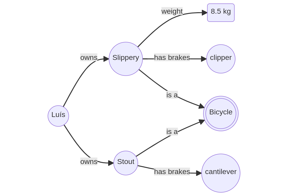
Note in the graph the different type of node used to express the “8.5 kg” literal. “Bicycle” is also expressed differently, with a double circle. That is to denote the difference between things, such as “Slippery” or “Stout” and categories of things. This is where semantics becomes relevant, as Chapter 3 shows in detail.
2.3 Turtle - Terse RDF Triple Language
RDF represents data with sets of interconnected triples that essentially state facts about a particular context. As Listing 5 exemplified, the linked nature of RDF provided by the employment of URIs makes the triples less than readable for humans. This in spite of the triple concept being rather similar to natural speech. A piece of the puzzle is missing: a syntax for the encoding (or expression) of triples. The end result must be something easily approachable by machines as well as humans.
In fact there are various options to this end, mostly specifications from the W3C. This book starts by introducing Turtle, short for the Terse RDF Triple Language (Beckett and Berners-Lee 2011). Of the different syntaxes available this is possibly the best for human consumption. It is also very similar to the syntax of the SPARQL query language (to be seen later in Chapter 5). Turtle is thus the best starting point for an introduction, but it is important to note that any RDF document described in this syntax can be automatically transformed into an alternative syntax.
2.3.1 Syntax basics
2.3.1.1 A triple
Defining a triple with Turtle is not that different from writing the
small sentences in natural language like in the previous section. A
Turtle triple is a sequence of three terms, the subject, the predicate
and the object, each separated by a white space and terminated by a full
stop (.). Some simple examples are given in Listing 6, in
the first line this is the subject, is_a the
predicate and triple the object. Triples always obey this
sequence in the Turtle syntax.
Listing 6: Simple triples expressed with the Turtle syntax.
this is_a triple .

another is_a triple .
This simple syntax is unlikely to ever produce any notable literary work, but it is easily readable by humans and interpretable by machines. A collection of these simple triples can gather a great deal of information.
2.3.1.2 URIs
But this is the Semantic Web, triple elements cannot be this simple,
they must either identify a resource or represent literals. Enter URIs
then. Turtle treats them as special citizens, enclosed within the
lower-than and greater-than characters (< and
>), for example:
<http://example.org/path/>. Listing 7 lays down the
same triples presented in Listing 6 but with URIs pointing to a
fictitious document. URI fragments differentiate the various
resources.
Listing 7: Triples expressed with URIs in the Turtle syntax.
<http://other.example.org/path#this> <http://example.org/path#is_a> <http://example.org/path#triple> .

<http://other.example.org/path#another> <http://example.org/path#is_a> <http://example.org/path#triple> .
URIs can also be relative references. Starting a URI directly with
the hash characters translates into a reference within the same document
or resource. For instance, the this and
another subjects could be referenced within the fictitious
document at http://other.example.org/path document defining
them as <#this> and
<#another>.
2.3.1.3 URI abbreviations
While the URI is a corner stone of the semantic web, by providing unique identifiers and the “linked” in “linked data”, they also make the encoding of RDF triples verbose and harder to read by humans. Moreover, URIs identifying resources within a same document are for the best past identical, they usually share the same URI schema and path, differing solely in the URI fragment. Full URIs not only clutter RDF documents, they also carry a good deal of redundancy.
Turtle deals with this problem in an elegant way, providing means for
the abbreviation of URIs. At the beginning of the document it is
possible to declare a particular string as an abbreviation for the lead
segment of an URI (usually the scheme and the path). This is made by
encoding a special triple with the keyword @prefix as the
subject, the abbreviation followed by the colon character
(:) as predicate and the abbreviated URI as object (Listing
8).
Listing 8: A URI abbreviation expressed in the Turtle syntax.
@prefix expl: <http://example.org/path#> .With the abbreviation defined, triple elements can be expressed in a
much leaner and readable way,
<http://example.org/path#this> becomes simply
expl:this. It is also possible to declare an empty
abbreviation, using solely the colon character as predicate. Empty
abbreviations are useful to shorten even further references to resources
within the same document. For instance with the abbreviation
@prefix : <http://example.org/path#> . the same
object can be expressed as :this.
The example in Listing 9 shows a full Turtle document that comes
closer to the way RDF is usually presented in this syntax. Abbreviations
are used as prefixes followed by the colon character and then the
resource name or identifier. A programme interpreting a Turtle document
automatically replaces the abbreviation followed by the colon with the
abbreviated URI. The URI segment figuring in the abbreviation
(e.g. http://example.org/path#) is also referred as
namespace.
Listing 9: A simple RDF document expressed in the Turtle syntax.
@prefix : <http://other.example.org/path#> .
@prefix expl: <http://example.org/path#> .

:this expl:is_a expl:triple .
:another expl:is_a expl:triple .
Note that in Listing 9 the predicate expl:is_a and the
subject expl:triple are defined in a different document.
Again, these RDF examples are still missing proper semantics, the topic
for Chapter 3.
2.3.1.4 Literals
The previous few sections were focused on the expression and location of resources with URIs, However, at some point data needs to come down to concrete information bits. In the Semantic Web and beyond these are known as literals. For the best part they are numbers and alfa-numeric strings, but there no actual limits to their nature.
In the Turtle syntax literals are always represented between double
quotes, for instance "triple name". Numbers are represented
in the same way, they do not differ from strings. Long strings
containing line breaks must be flanked by three double quote characters
("""). Listing 10 provides some basic examples.
Listing 10: Some RDF literals expressed in the Turtle syntax.
@prefix : <http://other.example.org/path#> .
@prefix expl: <http://example.org/path#> .

:this expl:is_a expl:triple .
:this expl:length "4" .
:this expl:name "This triple example" .
:this expl:description
      """ This is a long string describing the triple :this
          and also examplifying the encoding of long strings. """ .
2.3.1.5 Literal suffixes
Suffixes can be used to further specify the nature of literals. There are two kinds, suffixes declaring a language and suffixes declaring a literal type. They cannot be used together, as a language suffix only applies to strings.
Language suffixes are expressed with the at character
(@) followed by a language tag. Whereas the Turtle
specification itself does not make the nature of these tags explicit, it
is good practice to use the two character code list from the ISO 639-1
standard (“Codes for the representation of names of languages—Part
1: Alpha-2 code” 2002). Some examples are given in
Listing 11
Listing 11: Literal suffixes expressing the language of literals in the Turtle syntax.
@prefix : <http://other.example.org/path#> .
@prefix expl: <http://example.org/path#> .

:this expl:name "This triple example"@en .
:this expl:name "Ceci c'est un triple"@fr .
To specify a type other than string two circumflex characters
(^^) are used, followed by an URI locating the desired
definition. This URI can point to a particular type defined within an
ad hoc RDF document, or to one of the basic types identified in
the XML schema specification (Biron and Malhotra 2004). In any of
the cases, URI abbreviations can be used to declutter the encoding
(Listing 12). In Section 3.3.5 the literal types specified by the XML
schema are reviewed in more detail.
Listing 12: Literal suffixes expressing literal types in the Turtle syntax.
@prefix : <http://other.example.org/path#> .
@prefix expl: <http://example.org/path#> .
@prefic xsd: <http://www.w3.org/2001/XMLSchema#> .

:this expl:length "4"^^xsd:integer .
:this expl:type "short"^^<http://example.org/path#tripleType> .
2.3.1.6 Comments
Comments can be introduced anywhere in a Turtle document. They can be
used to identify the document author, its purpose, relation to other
documents, etc. They can annotate certain elements and provide cues on
their meaning. A comment is inserted with the hash character
(#), whatever is written after it in the same line is
ignored. E.g. # This is a comment.
2.3.2 Triple Abbreviations
One of the goals in the Turtle syntax is to declutter the encoding of triples. Earlier you saw how abbreviating URIs helps in achieving an easily readable RDF document. But abbreviations go further, with Turtle it is possible to abbreviate triples themselves.
2.3.2.1 Abbreviate subject and predicate
Data in digital form are often formed by sets of characteristics
describing a certain object. Just like each row in a CSV file or
database table provide diverse information bits related to a same
entity, object, person, etc. Such kind of data translates into RDF with
sets of triples with the same subject, or even with the same subject and
predicate, take for instance Listing 13. Turtle allows the abbreviation
of this kind of triples, instead of declaring only one object for the
subject–predicate pair, the comma character (,) can be use
to encode a list of different objects. Listing 14 gives an example that
encodes the exact same triples as Listing 13. It is common to declare
each subject in its own line, to ease reading further.
Listing 13: Example RDF triples with repeated object and predicate.
@prefix : <http://other.example.org/path#> .
@prefix expl: <http://example.org/path#> .

:this expl:is_a expl:triple .
:this expl:is_a expl:example .
:this expl:is_a expl:simple .
Listing 14: Example RDF triples with abbreviated object and predicate in the Turtle syntax.
@prefix : <http://other.example.org/path#> .
@prefix expl: <http://example.org/path#> .

:this expl:is_a expl:triple ,
                expl:example ,
                expl:simple .
2.3.2.2 Abbreviate subject
A similar strategy is used to abbreviate triples that share the same
subject (but not the same predicate). In this case the semi-colon
character (;) is used to provide a list of predicate–object
pairs. Consider again Listing 12, that provided the example with
literals. Since both triples have the same subject, they can be
abbreviated as Listing 15 shows. Note again the practice of encoding
each predicate–object pair in its own line.
Listing 15: Example RDF triples with abbreviated object in the Turtle syntax.
@prefix : <http://other.example.org/path#> .
@prefix expl: <http://example.org/path#> .
@prefic xsd: <http://www.w3.org/2001/XMLSchema#> .

:this expl:length "4"^^xsd:integer ;
      expl:type "short"^^expl:tripleType .
2.3.3 Collections
The RDF standard specifies a special kind of object for lists of
things: the collection. It is a recursive construct, the first element
is declared with the rdf:first predicate and the remainder
as a sub-collection, using the rdf:rest predicate. With all
elements declared, the rdf:nil predicate is used to close
the collection. In the Turtle syntax, lists are enclosed with square
brackets ([ and ]) with individual elements
separated by a semi-colon (;). Listing 16 shows an
example.
Listing 16: RDF triples encoding a collection in the Turtle syntax.
@prefix : <http://other.example.org/path#> .
@prefix expl: <http://example.org/path#> .
@prefix rdf: <http://www.w3.org/1999/02/22-rdf-syntax-ns#> .

:this expl:has_list [ rdf:first "Element A";
                      rdf:rest [ rdf:first "Element B";
                      rdf:rest [ rdf:first "Element C";
                      rdf:rest rdf:nil ] ] ] .
That is a good deal of text to declare a list composed by three
simple literals. Turtle thus allows abbreviating collections further, by
directly enclosing elements in brackets (( and
)), separated solely by empty spaces. Listing 17 below
encodes exactly the same information as Listing 16 but is far more
readable. The tautology from this syntax is that ( ) is an
abbreviation for rdf:nil.
Listing 17: RDF triples enconding a collection in Turtle with abbreviated syntax.
@prefix : <http://other.example.org/path#> .
@prefix expl: <http://example.org/path#> .
@prefix rdf: <http://www.w3.org/1999/02/22-rdf-syntax-ns#> .

:this expl:has_list ( "Element A" "Element B" "Element C" ) .
2.3.4 Blank nodes
Look carefully again at Listing 16. Perhaps you noticed before, inside the square brackets there are no triples, but rather doubles. How can that be? They are in fact triples but their object is invisible, what in the Semantic Web is known as a Blank Node. The concept of blank node is general to RDF but is perhaps best exemplified with the Turtle syntax. In essence it is a shortcut to lean out and simplify documents. The blank node results from a collection of triples referring all to the same subject. For the sake of brevity, RDF allows the expression of such triples without explicitly declaring the subject. The programme that later reads the RDF is then responsible for creating a logical identifier for the subject.
With the Turtle syntax, a blank node is declared within a square
brackets block. Inside the block are pairs of predicates and subjects,
separated by a semi-colon (;). Listing 18 provides an
example. The usefulness of blank nodes will become more evident once you
learn how to specify an ontology (Chapter 3).
Listing 18: Blank nodes in the Turtle syntax.
@prefix rdf: <http://www.w3.org/1999/02/22-rdf-syntax-path#> .
@prefix dc: <http://purl.org/dc/elements/1.1/> .
@prefix ex: <http://example.org/stuff/1.0/> .

<http://www.w3.org/TR/rdf-syntax-grammar>
  dc:title "RDF/XML Syntax Specification (Revised)" ;
  ex:editor [
    ex:fullname "Dave Beckett";
    ex:homePage <http://purl.org/net/dajobe/>
  ] .
2.3.5 The “Slippery” example
Closing this Section, Listing 19 presents the “Slippery” triples again, but in the Turtle syntax. The same facts are stated again with URIs, but in a way that almost resembles the initial natural language statements. Machine and human readable.
Listing 19: The triples about the Slippery bicycle expressed in the Turtle syntax.
@prefix : <http://www.linked-sdi.com#> .

:Slippery :is_a :bicycle ;
          :has_brakes :caliper ;
          :weight_kg "8.5" .

:Luís :owns :Slippery .
2.4 Other RDF syntaxes
The Turtle syntax is one of many specified the past decades. This
section provides brief examples of alternative syntaxes that are also
relevant. They are not presented in detail like Turtle, it is instead
important to retain their existence. Do not shy away if you come across
RDF triples in what appears a foreign syntax. An online tool like the
one provided by isSemantic.net 3 can
easily translate to a familiar syntax. For the remainder of this
manuscript only Turtle will be used, as at present this is possibly the
leanest and easier to read by humans.
2.4.1 RDF/XML
RDF was initially specified on a XML syntax, first published by the
W3C in 2001 and updated several times up to version 1.1 released in 2014
(Gandon and Schreiber
2014). This syntax is today better known as RDF/XML. It is not
the most user friendly syntax and also rather verbose. RDF documents are
encoded as series of rdf:Description sections, each
reporting triples for a single subject. The latter is identified with
the rdf:about annotation in the opening section statement.
Each triple predicate translates into an independent statement within
the rdf:Description section
(e.g. <has_brakes in Listing 20). Objects of the type
resource are encoded with a rdf:resource annotation,
whereas literals get their own statement (e.g.
<weight_kg> in Listing 20). RDF/XML introduced the
concept of annotations (and namespaces) to RDF encoding, in that sense
helping to lean documents. However, with the formal sections and
statements and the full encoding of subject URIs it can still produce
rather cluttered documents for human eyes. Listing 20 encodes the
Slippery triples originally given in Listing 19. Compare the size of
both documents.
Listing 20: The triples about the Slippery bicycle expressed in the RDF/XML syntax.
<?xml version="1.0" encoding="UTF-8"?>
<rdf:RDF
   xmlns="http://www.linked-sdi.com#"
   xmlns:rdf="http://www.w3.org/1999/02/22-rdf-syntax-ns#"
>
  <rdf:Description rdf:about="http://www.linked-sdi.com#Slippery">
    <weight_kg>8.5</weight_kg>
    <has_brakes rdf:resource="http://www.linked-sdi.com#caliper"/>
    <is_a rdf:resource="http://www.linked-sdi.com#bicycle"/>
  </rdf:Description>
  <rdf:Description rdf:about="http://www.linked-sdi.com#Luís">
    <owns rdf:resource="http://www.linked-sdi.com#Slippery"/>
  </rdf:Description>
</rdf:RDF>
2.4.2 N-Triples
N-Triples is a syntax developed about a decade ago, in parallel to
Turtle. Whereas the former intended to make RDF succinct and easy to
read by humans, N-Triples targeted ease of read by machines (Beckett, Carothers, and
Seaborne 2014). The concept is simple, each line corresponds to a
triple, with subject, predicate and object separated by a blank space
and URIs delimited by lower and greater characters (<
and >). A full stop (.) marks the end of a
triple. To a human the N-Triples looks very much like Turtle, but
without abbreviations. While N-Triples indeed facilitates triple
encoding/decoding by software it is also one of the most verbose RDF
syntaxes. Listing 21 presents again the Slippery triples in this
syntax.
Listing 21: The triples about the Slippery bicycle expressed in the N-Triples syntax.
<http://www.linked-sdi.com#Slippery> <http://www.linked-sdi.com#has_brakes> <http://www.linked-sdi.com#caliper> .
<http://www.linked-sdi.com#Slippery> <http://www.linked-sdi.com#weight_kg> "8.5" .
<http://www.linked-sdi.com#Slippery> <http://www.linked-sdi.com#is_a> <http://www.linked-sdi.com#bicycle> .
<http://www.linked-sdi.com#Lu\u00EDs> <http://www.linked-sdi.com#owns> <http://www.linked-sdi.com#Slippery> .
2.4.3 JSON-LD
Soon after N-Triples and Turtle the W3C published yet another RDF
syntax, this time with web programming in mind. JSON-LD (Sporny et al. 2020) is a
RDF syntax leveraged on the JSON file format, thus directly translatable
to assets like objects and lists in programming languages such as
JavaScript or Python. A JSON-LD is usually outlined with two sections,
one with the context (@context object) encoding
abbreviations, and another for the actual triples (@graph
object). A JSON object is created for each subject, with respective
predicates and objects encoded as dictionaries (i.e. key-value pairs).
List may be used to link more than one subject with the same predicate.
Visually, JSON-LD is not a cluttered syntax (e.g. compared with
RDF/XML), but carries many bracket and curly bracket characters that can
make for a challenging read, especially in longer documents. Listing 22
provides an impression of this syntax for the Slippery triples with a
few exemplary abbreviations. JSON-LD makes extensive use of the JSON
specification, with plenty of alternatives for special cases. Among
other things, it is possible to define object-specific context sections,
that apply to a single subject. For the purpose of this manuscript this
early contact with JSON-LD is enough, however, if you ever intend to
work with RDF in a programming context a deeper understanding of this
syntax may come handy, especially in a web oriented environment.
Listing 22: The triples about the Slippery bicycle expressed in the JSON-LD syntax.
{
  "@context": [
    {"is_a": "http://www.linked-sdi.com#is_a"},
    {"has_brakes": "http://www.linked-sdi.com#has_brakes"},
    {"weight_kg": "http://www.linked-sdi.com#weight_kg"},
    {"owns": "http://www.linked-sdi.com#owns"}
  ],
  "@graph": [
   {
    "@id": "http://www.linked-sdi.com#Slippery",
    "is_a": "http://www.linked-sdi.com#bicycle",
    "has_brakes": "http://www.linked-sdi.com#caliper",
    "weight_kg": "8.5"
   },
  {
    "@id": "http://www.linked-sdi.com#Luís",
    "owns": [{
        "@id": "http://www.linked-sdi.com#Slippery"
      }]
  }]
}
2.4.4 Notation3
Just a few years after starting the development of the Turtle syntax, the W3C housed its evolution into what became known as Notation3 (Tim Berners-Lee and Connolly 2011) (or N3 for short). This syntax expanded on Turtle aiming to facilitate further the expression of lists, logics or variables. Since it expands on Turtle, the triples in Listing 19 would not look any different in Notation3. However, Notation3 is well worth mentioning for it is actually an attempt to expand on RDF itself. It proposes new concepts such as functional predicates or literals that express whole graphs. Perhaps due to these ambitious goals, N3 never made it to an actual W3C recommendation, and has not been updated since 2011. However, it can be the root for new developments in the Semantic Web, that will be relevant to follow upon.
2.5 RDF Schema
From the onset the W3C meant to lend a semantic dimension to RDF. Accompanying the RDF specification the W3C also developed the RDF Schema Specification (RDF Schema or RDFS for short) (Brickley and R. V. Guha 1999). This specification had several goals: provide a best practice for the general structure of knowledge graphs, to standardise the linkage between knowledge and resources and be the basis for the semantic expression of RDF.
RDFS is a relatively compact set of general classes or categories of resources plus a set of predicates. All these resources are defined in two RDF documents maintained by W3C:
http://www.w3.org/1999/02/22-rdf-syntax-path#(abbreviated tordf:)http://www.w3.org/2000/01/rdf-schema#(abbreviated tordfs:)
The most relevant are briefly described next.
2.5.1 Categories
RDFS specifies a set of categories of resources, creating an elementary framework to differentiate objects (and subjects) in a knowledge graph. It considers the distinction between a resource proper and a literal, and some more. The most relevant are:
rdfs:Resource: the category of all things, as everything in RDF is a resource.rdfs:Class: specifies a particular category of resources. The meaning of the term Class is explained in detail in Section 3.2.rdfs:Literal: everything which is not a resource identifier, in most cases strings and numbers. Literals may have a type.rdfs:Datatype: the category of all literal types.
2.5.2 Predicates
A small, but powerful, set of predicates provides basic mechanisms to link to other resources and knowledge graphs in a standardised way. It also adds basic constraints to the formation of triples. Those deserving to be highlighted at this stage are:
rdfs:domain: used to specify the category of the object in a triple.rdfs:range: used to specify the category of the subject in a triple.rdf:type: declares a particular resource as being an element of a category. Can be abbreviated further toa.rdfs:label: provides a human readable name for a resource.rdfs:comment: annotates a resource with a human readable description.rdfs:seeAlso: links a resource to another resource that provides more information, or that is somehow related.rdfs:isDefinedBy: links a resource that defines the subject further.
2.5.3 The “Slippery” example
The simple example with the “Slippery” bicycle is again a good case
to show how RDFS can be used. Listing 23 expands on Listing 19 with the
addition of various triples that start making this knowledge graph truly
Linked Data. Take some time to study all the new triples.
Bicycle is now defined as a category of resources (or
things), with name, a brief description and a link to an external
resource, in this case a Wikipaedia page. Slippery is also
upgraded, with a formal name and description and a link back to its
owner. Note also the use of the a predicate to define
Slippery as a Bicycle.
Listing 23: The triples about the Slippery bicycle expanded with RDFS.
@prefix rdf: <http://www.w3.org/1999/02/22-rdf-syntax-path#> .
@prefix rdfs: <http://www.w3.org/2000/01/rdf-schema#> .
@prefix : <http://www.linked-sdi.com#> .

:Bicycle rdf:type rdfs:Class ;
         rdfs:label "Bicycle" ;
         rdfs:comment
              """A light-weight, pedal-powered vehicle
                 with two wheels attached to a frame,
                 one after the other.""" ;
         rdfs:isDefinedBy <https://en.wikipedia.org/wiki/Bicycle> .

:Slippery a :Bicycle ;
          rdfs:label "Slippery" ;
          rdfs:comment
               "A road sports bicycle with caliper brakes." ;
          rdfs:seeAlso :Luís ;
          :has_brakes :caliper ;
          :weight_kg "8.5" .

:Luís :owns :Slippery .
In a real knowledge graph it would be necessary to define the meaning
(i.e. semantics) of the predicates :has_brakes,
:owns, etc., and also the objects :Luís and
:caliper. If you never worked with data semantics before
things may start to seem too abstract at this stage. Fear not, Chapter 3
provides a thorough introduction to the Web Ontology Language, the W3C
standard that built on RDFS towards rich data semantics.
3 Web Ontology Language
The previous chapters were concerned with the syntax of Linked Data. The basic ways to represent data with RDF and the core standards making data “linked” on the internet. This chapter now dives into the semantics, how data is invested with meaning that is formalised and therefore unequivocal. That is the role of ontologies, abstractions of the real world synthesising concepts humans employ in natural discourse. The Web Ontology Language is the keystone of the Semantic Web, as it fulfils this capital role of formalising semantics, i.e. the meaning and intent of each datum.
This is the most abstract chapter in this book, and could be the most challenging for some readers. While you may never need to develop an ontology, at the end of the chapter you should be able to identify the set of ontologies relevant to a particular domain and how to apply them correctly. Understanding the basics of OWL and how to use ontologies is also crucial for geo-spatial data in the Semantic Web and the associated meta-data.
3.1 Historical Notes
Industries understood the power of computers to process data soon after World War II. Business oriented hardware and software proliferated throughout the 1950s, at first without coordination between vendors. In 1959, several companies in the United States assembled a consortium around CODASYL (Conference on Data Systems Languages) with the purpose of defining a programming language for data systems that could be executed on multiple hardware platforms. One of the results was the COmmon Business-Oriented Language (COBOL) programming language. If at first it had little clout with the software industry, once it was made mandatory by the United States government (Ensmenger 2012) it became a de facto standard.
Data stored by computers those days amounted to little more than collections of files, each storing a set of records. Soon enough industrial and governmental information systems grew in complexity past such simple structures. As the 1970s dawned, various attempts emerged towards more abstract and complex ways to represent data stored by computers. Eventually, (Chen 1976) proposed the Entity-Relationship (ER) meta-language, that finally broke in as a popular choice. Entity is something that exists, a being or a particular unit, relationship is a connection or association. ER is a graphical language, providing constructs to express categories of data, their attributes and the relationships between categories (Figure 3). While simple, ER completely abstracts the description of data from the underlying software or hardware.
Chen’s choice of words was not at hazard. In 1970, Codd had introduced the concept of “relational database”, defining rules for data management software that went beyond earlier file-based systems (Codd 1970). The first implementation of Codd’s vision was released in 1976 by IBM, the Multics Relational Data Store (Van Vleck 2023). In 1979, a small company named Relational Software released a relational database management system named Oracle, which grew enough to even take over the name of the company. ER and relational databases proved a perfect match, providing the theoretical and practical facets to data management. Together they swept the software industry and computer science curriculae.
In 1967, researchers at the Norwegian Computing Centre introduced a language for computer simulation – Simula – that included the concepts of objects, classes of objects and class inheritance (these are explored in more detail in the following section) (Dahl and Nygaard 1966). Simula was not a success with the industry, but proved immensely influential on subsequent programming languages. In 1980, Smalltalk was released, product of an effort at Xerox towards an educational programming language (Goldberg and Robson 1983). Smalltalk not only adopted the concept of objects from Simula, it made them its central paradigm (a sample programme is in Listing 24). By the middle of the 1980s the introduction of industry grade languages like C++ and Eiffel made object-oriented programming a staple of software development.
Listing 24: A sample programme in the Smalltalk language. Declares a class with a method to print a message, then instanciates the class and invoques its method.
Object subclass: #Hello
    instanceVariableNames: ''
    classVariableNames: ''
    package: 'SmalltalkExamples'

Hello>>sayHello
    Transcript show: 'Hello World!'

Hello new sayHello
At the dawn of the 1990s a more fundamental understanding of software development came about. First Powers (Powers 1991) and then Gruber (Gruber 1995) proposed the direct application of Ontology to computer science. The term ontology became first popular within the artificial intelligence community and later in computer science to signify an abstract representation of real-world concepts pertaining to a particular domain or field.
The rapid growth of object-oriented programming fuelled the demand for novel abstract means to develop and document software. Rumbaugh et al. (Rumbaugh et al. 1991) and Booch (Booch et al. 2008) proposed the earliest infrastructures towards this end. Reunited under the Rational Software Corp. these and other researchers would develop such concepts into the Unified Modelling Language (UML). UML matched object-oriented programming just as ER had matched relational databases two decades earlier. But UML is a far more powerful and extensive language, allowing the abstraction of a wide range of constructs, such as class inheritance and composition, all with an expressive graphical meta-language. UML largely provided the infrastructure for applied philosophy envisioned by Powers and Gruber. UML was adopted as a standard by the Object Management Group (OMG) in 1997, at a time when it already featured at large in computer science curriculae.
At the turn of the 21st century, the UML standard was pushed into an even higher level of abstraction. In 2003, the IEEE Software journal published a series of articles advocating a novel software development method named Model-Driven Development (MDD) in which domain models are the primary products, and source code is a by-product Selic (2003). This idea was not entirely new, as various companies had since the 1980s proposed software to generate source code from graphical models (commonly known as CASE tools). What MDD brought anew was the extension of UML into meta-modelling, using abstractions such as categories of categories to capture the essential aspects of a knowledge domain. A broader discipline covering MDD, CASE tools and more became known as Model-Driven Engineering (MDE) (Da Silva 2015).
In 2005, UML version 2.0 was released, including an entire infrastructure (primitives and methods) dedicated to meta-modelling named Model-Driven Architecture (MDA) (Soley et al. 2000). With MDA, the core UML primitives can be specialised through a special primitive: the stereotype. A semantically related set of stereotypes can be gathered into a UML Profile, thus constituting a domain-specific lexicon, i.e. an ontology. MDA was almost immediately adopted by the industry and has since been used by various institutions to issue standards. Noteworthy are those issued by the Open Geospatial Consortium (OGC), many of which were also adopted by ISO. The INSPIRE domain model is also specified with the MDA infrastructure.
In parallel to the efforts of the OMG, the World Wide Web Consortium (W3C) also worked towards an ontology infrastructure. The W3C was primarily concerned with the exchange and automatic processing of data in the age of the internet. It started by specifying the RDF Schema, encompassing basic ontological notions such as category (class), property (domain, range, etc) and inheritance (sub-class).
When the first full RDF specification was released in 2004, the W3C had already started working on a more abstract infrastructure for meta-modelling. With a purposeful name, Web Ontology Language, and a catchy acronym, OWL, it presented a novel approach to ontology modelling (McGuinness, Van Harmelen, et al. 2004). OWL is not as abstract as UML, resulting from a process focused on the practical aspects of data exchange over the internet. The Semantic Web is yet to reach the ubiquity of UML and MDA, but as Chapter 1 outlined, modern requirements for data exchange might well change that picture.
3.1.1 Terminology
Before moving on to the theory it is important to pin down the terminology around Ontology employed in this manuscript. The definitions below large match the common interpretation of these terms in computer science. If something is not yet fully clear do not worry, the subsequent sections have the details.
Ontology: written with capital “O” refers to the branch of Metaphysics providing the general concepts used to abstract information in computer science.
ontology or information ontology: written with small “o” refers an abstract representation of a real world domain, using Ontology principles, and applicable in computer science. A ER or a UML model can be examples.
web ontology: an ontology (with small “o”) expressed with the Web Ontology Language.
3.2 Ontology
Sometime in the V century BC the Greek philosopher Parmenides wrote a poem. It was possibly titled “On Nature”, delving into broad questions on how humans perceive and interpret the reality around them. Much of the text was lost in the subsequent millennia, but Parmenides’ impact on the emergence of Ontology as a novel branch of Metaphysics prevails to this day. Eventually it would have a decisive impact on computer science, as Section 3.1 laid out.
Ontology has underwent twists and turns through history and retains a myriad of unresolved dissensions. It is therefore important to realise that the concepts absorbed in computer and information science are not universally accepted within the Ontology discipline itself. However, they enclose the metaphysical principles supporting the development and modelling of information ontologies.
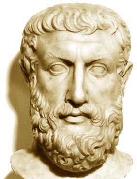
A core idea of Ontology is the contrast between universals and particulars (Honderich 2005a). A universal is a category of entities that can be exemplified by various particulars. A particular is an entity that can usually be sited at a particular time and point in space. Universals are therefore more conceptual (or metaphysical) and particulars more physical. For instance, the idea of “Bicycle” is a universal, a category of vehicles with particular characteristics: two wheels, two pedals, a seat and a steering set. Whether you invoke that concept in Europe or in Africa, it translates into a somewhat similar abstraction in the mind of whom listens. It is not possible to site the generic idea of “Bicycle” in space or time. In contrast, the two bicycles I referenced before, “Slippery” and “Stout” are particulars. I can inform you where they are now and where they were a span of time ago. I can also inform you on their colours, their weight and other characteristics. “Slippery” and “Stout” are physical, whereas “Bicycle” is abstract.
In information and computer sciences (Figure 5), universals mostly appear with the name Class, a term common to both UML and OWL (in the earlier ER meta-model these where the Entities). A Class is a category of entities that share a common set of characteristics. In MDA and object-oriented programming, particulars are known as “instances”, “class instances” or “objects”. In the Semantic Web, particulars are more often called “individuals”, a term that is also found in Ontology. The concept of Class in UML is somewhat broader since it can also specify behaviours that are common to its instances. However, this aspect is more relevant to programming than information science per se.
A further core concept in Ontology is that of “property” (Orilia and Paolini Paoletti 2020) which is employed in similar sense in information science. A property conveys a specific characteristic of its bearer, expressing what the bearer is like. In information science, both universals and particulars have properties. At the universal level, they express a type of feature, whereas for the particular they assign a concrete value to that feature. You have seen this already in Section 2.2. Being an universal, “Bicycle” has the “weight” property (or weight in kg, to be more precise). The particulars instantiate that property with “8.5” in the case of “Slippery”, and “13” for “Stout”. Properties in the Semantic Web and MDA have a determined type, usually an atomic computer system type (i.e. floating point, string), or a combination of these.
Another Ontology concept taken literally in information science is that of “relation” (or “relationship”) (Honderich 2005b). Relations express how different entities stand to each other. This term gave the name to the Entity-Relationship meta-model but is often referred as “association”, particularly in UML. In information science, relations have the critical facet of “cardinality”, already present at the time of ER. With cardinalities, information ontologies express how many particulars of a certain universal can relate to one particular of another universal. Again recalling the triples in Section 2.2, there was an implicit relation between “Bicycle” and “Person”, named “owns”. A formal relation can specify that a bicycle is owned by a person, and that a person can own various bicycles. Therefore “Slippery” is owned by “Luís”, and “Luís” owns both “Slippery” and “Stout”. Cardinalities are essential to structure storage and validate data in computer systems.
Other Ontology concepts were absorbed in a less straightforward fashion in information science. Most relevant among these is ontological dependence (Tahko and Lowe 2020), stating that certain entities cannot exist without the existence of another (usually related) entity. Ontological dependence is sub-divided into sub-concepts: rigid dependence, that refers to a specific particular, and generic dependence, referring to a category of particulars (or universal). In the Semantic Web rigid dependence is usually expressed through cardinalities in relations. However, UML provides a specific construct akin to rigid dependence named “composition”.
Generic dependence appears in information science in the form of class hierarchies. It features prominently in OWL and UML, signifying that a child class yields all the same properties and behaviours of its parent class. The universals “Bicycle” and “Tricycle” express different concepts, but share a number of similar features: both have pedals and a steering set, both can go on cycle paths. Thus the common properties to these two universals can be generalised by a parent universal named “Pedal Vehicle”. This feature is referred by the names “inheritance” and “generalisation” in information science. The Ontology discipline also conceives generic dependence as a vehicle to hierarchic structuring, distinguishing between more fundamental entities and secondary ones.
Table 4 provides a quick reference for these main concepts of Ontology absorbed in computer science and used at large in the Semantic Web. In Section 3.3 these concepts will become more concrete, with examples on how to formalise them with the Web Ontology Language.
| Concept | Description | Also known as |
|---|---|---|
| Universal | An abstract idea, a category of things. | Class |
| Particular | The instance of a universal, a physical thing. | Instance |
| Property | A characteristic of a universal, instantiated by particulars. | |
| Relation | Expresses how universals and particulars stand to each other. | Association, Relationship |
| Cardinality | Limits relations between particulars of two universals. | |
| Generalisation | Structures universals in a hierarchy. | Inheritance, Generic dependence |
3.3 Primitives of the OWL
3.3.1 An Ontology with OWL
The best way to introduce OWL is with an example. The “Slippery” triples illustrating Section 2.2 provide the motto for a web ontology about bicycles and similar vehicles. For simplicity it is called “Mobility” and gathers basic axioms to describe and categorise bicycles with RDF and relate them to other categories, like owners. A complete rendition of this ontology in Turtle is available in Annex A, it will be used throughout the manuscript and later augmented with geo-spatial concepts.
The first axiom to use is the declaration of an ontology itself. OWL
provides a specific class (or category) for that: Ontology.
Listing 25 provides the very first lines of a web ontology, declaring
the document as such, and using RDFS predicates to convey a basic
description. Beyond a simple name and description, a URI for the
ontology itself is declared in Listing 25, in this case
https://www.linked-sdi.com/mobility# . This corresponds to
the actual location of the Mobility ontology on the manuscript web page.
It is important to devise the appropriate URI for an ontology or a
knowledge graph, a topic discussed in more detail in Chapter 8.
Likewise, providing meta-data on the ontology itself is important to
whomever comes to use it, the topic for Chapter 9. Step by step you will
come to understand all these aspects of the Semantic Web, but at this
stage the focus is on OWL.
Listing 25: An ontology declared with OWL
@prefix : <https://www.linked-sdi.com/mobility#> .
@prefix owl: <http://www.w3.org/2002/07/owl#> .

: rdf:type owl:Ontology ;
  rdfs:label "Mobility ontology"@en ;
  rdfs:comment
       """ An illustration ontology to describe human powered
           vehicles, their owners and ways of use."""@en .
Note again the second line in Listing 25, it abbreviates the general
URI of the OWL specification. Experiment opening the URI with your web
browser. The first triple in the document is
<http://www.w3.org/2002/07/owl> a owl:Ontology.. OWL
is itself an ontology, or better worded, a meta-ontology, an ontology
for the specification of ontologies.
3.3.2 Classes and instances
The Class is the most essential element of a data structure, called Universal in Ontology, and also known as Category in mathematical logics. A Class represents a set of things or entities that share some sort of similarity, either in their properties, their state or their behaviour. In information science and computer science particulars of a class are better known as instances, so that term is favoured in this text.
In Section 2.2 there was already a concrete example of the contrast between class and instance with the declaration of “Slippery” as a “Bicycle”. In practice this means “Slippery” is an instance of the “Bicycle” class. “Stout” is my city bike, therefore “Stout” is also an instance of “Bicycle”. At any moment I should be able to tell where “Stout” and “Slippery” are, but not “Bicycle”. It is rather an umbrella term for human-powered vehicles with two longitudinal wheels. “Stout” and “Slippery” are different from each other, but share a number of characteristics.
The declaration of a class is thus one of the basic axioms of an
ontology. In OWL this is made with a triple whose subject is the
declared class, the object is the OWL element class and the
RDF predicate type. In Listing 26 a new class named
Bicycle is declared in this way.
Listing 26: A class declaration with OWL
@prefix : <https://www.linked-sdi.com/mobility#> .
@prefix owl: <http://www.w3.org/2002/07/owl#> .
@prefix rdf: <http://www.w3.org/1999/02/22-rdf-syntax-ns#> .

: rdf:type owl:Ontology .

:Bicycle rdf:type owl:Class .
By itself, Listing 26 is already the archetype of an ontology, as it declares the existence of a Class specific to some domain. Saving it as a Turtle file and exposing it through an HTTP service would be enough to start using it. The details will be addressed in subsequent chapters, first the ontology needs to grow into something more explicit.
3.3.3 Class instances and identifiers
If you are familiar with information science you are probably aware of the importance of unique identifiers. They are essential to tell one information bit from another, be it a line in a text file or a row in a relational database table. Identifiers are usually integer numbers, sometimes text strings are used, in more sophisticated systems UUIDs can also be found.
From an ontological perspective, identifiers are characteristics that
unequivocally locate the instances of a Class. In the context of the
Semantic Web, identifiers are provided by default as URIs. Have another
look at Listing 26, the definition of the Bicycle class
creates a URI: http://www.linked-sdi.com/mobility#Bicycle.
Likewise, the declaration of an instance of that class automatically
creates a unique, and universal, identifier. Take for instance the
example of Listing 27 in which two instances of Bicycle are
declared:
Listing 27: Instances of the Bicycle class declared with OWL
@prefix : <http://www.linked-sdi.com/vehicles#>
@prefix mob: <http://www.linked-sdi.com/mobility#> .
@prefix rdf: <http://www.w3.org/1999/02/22-rdf-syntax-ns#> .

:slippery rdf:type mob:Bicycle

:stout rdf:type mob:Bicycle
Slippery and Stout thus become automatically
identified with the URIs
http://www.linked-sdi.com/vehicles#slippery and
http://www.linked-sdi.com/vehicles#stout.
The practical result is that you do not need to declare explicit Class identifiers in OWL. Be it a classical auto-increment integer or a textual name or label. Class instances in the Semantic Web are uniquely identified by nature. Thus ontology development can focus exclusively on the actual semantics and specifics of the domain.
3.3.4 Class properties and literal types
Properties extend classes with the means to specify the characteristics of each of its individuals. Each individual of a class assigns precise values to the properties defined. Properties thus allow to distinguish and characterise each individual.
Consider again the Bicycle class example, with the two
individuals, Slippery and Stout. Not everyone is
addicted enough to name their bicycles, so let us consider more
practical properties to distinguish between them, like
colour, size or weight.
Splippery is black and white, whereas Stout is all
black, Slippery’s frame is 56 cm, whereas Stout’s is
57 cm. Slippery is light, well under 10 kg, Stout is
much heavier, some days feels like a tonne.
Coming down to the OWL idioms, class properties are declared with the
OWL class DatatypeProperty, in similar fashion to class
declarations. Then a domain and a range must be declared. The former
declares the class to which the property belongs, the latter indicates
the type of values that can be associated with the property. Generally,
ranges are literal types. Listing 28 declares the data type properties
colour, size and weight for the
Bicycle class. Note again how the Turtle language is used
to simplify the predicates pertaining to a same subject. The following
section provides more details regarding the literal types that can be
used with OWL.
Listing 28: Class property declarations in OWL
@prefix : <http://www.linked-sdi.com/mobility#> .
@prefix owl: <http://www.w3.org/2002/07/owl#> .
@prefix rdf: <http://www.w3.org/1999/02/22-rdf-syntax-ns#> .
@prefix rdfs: <http://www.w3.org/2000/01/rdf-schema#> .

:colour rdf:type owl:DatatypeProperty ;
    rdfs:domain :Bicycle ;
    rdfs:range xsd:string .

:size rdf:type owl:DatatypeProperty ;
    rdfs:domain :Bicycle ;
    rdfs:range xsd:integer .

:weight rdf:type owl:DatatypeProperty ;
    rdfs:domain :Bicycle ;
    rdfs:range xsd:real .
3.3.5 Literal types
Following on its logic of reusing existing infrastructure and standards as much as possible, the W3C did not define new types specific to OWL. It rather adopted those already defined for XMLSchema (Biron and Malhotra 2004), all of which can be used in an ontology described with OWL. Among these types there are some very specific to computer science, but familiar types matching simple data literals expressed with character strings and numbers are available. A list of the most relevant:
xsd:string- the usual character string literals composed by text, e.g. the colour of an object.xsd:boolean- the building block of logic, “true” or “false”, “on” or “off”.xsd:dataTime- for literals that express a point in time.xsd:integer- a natural number, i.e. without decimal fraction.xsd:float- a floating point number, i.e. integers, decimals and real numbers (e.g. square root of 2). The term “float” in computer science implies a 32-bit number, which limits the range of real numbers this type can represent. Thus there is alsoxsd:doublefor 64-bit real numbers, and OWL includes theowl:realtype for a broader definition.xsd:anyURI- a URI identifying a resource. Both absolute and relative URIs are acceptable, as are fragments in a resource (using the character#).xsd:Name- an XML name. It represents a character string with specific limitations: it must start with a letter, an underscore or a colon, and may only contain letters, digits, underscores, colons, hyphes and periods.owl:real- a real number, including all naturals, quotients and rational numbers.
The RDF Schema specification extends the XML Schema with a few more literal types. Two of these can be highlighted:
rdf:XMLLiteral- a fragment of an XML document. This type is used to embed XML within a RDF dataset.rdf:JSON- a fragment of a JSON document. Used to embed JSON within a RDF dataset.
3.3.6 Literals facets
An indispensable aspect defining an ontology is the ability to set
limitations or boundaries to literals used to describe the properties of
an individual. For instance, :weight was earlier declared
as a real number, but not all real numbers can describe the weight of a
bicycle. A bicycle individual with a negative weight is not a very
useful piece of data, it is likely wrong.
Declaring the type of a property sets a constraint to what kind of
literals can be used to instantiate the corresponding class. If
:size is of type xsd:integer it cannot be
matched with the literal “A”, for instance. However, in this (and many
similar circumstances) it is necessary to set more specific limitations
or boundaries to literals used to describe the properties of an
individual. Therefore, it is useful not only to declare the type of a
literal but also restrict is range. In the world of the Semantic Web
these restrictions can be set with a mechanism know as literal facets.
They are similar to the logic restrictions applied to individual fields
in a relational database. More specifically, the
owl:withResctrictions predicate is used to list one or more
literal facets applicable to the property in question. This extra
predicate has an implication: the property range must itself become a
structured element.
Coming back to the Bicycle example, say you want to limit the range
of values for the :weight property. It should not be under
the UCI’s legal limit, and also it should not be over 30 kg4. Listing 29 shows how to it can be
done.
Listing 29: OWL facets limiting the range of a DatatypeProperty.
@prefix : <http://www.linked-sdi.com/mobility#> .
@prefix owl: <http://www.w3.org/2002/07/owl#> .
@prefix xsd: <http://www.w3.org/2001/XMLSchema#> .
@prefix rdf: <http://www.w3.org/1999/02/22-rdf-syntax-ns#> .
@prefix rdfs: <http://www.w3.org/2000/01/rdf-schema#> .

:weight rdf:type owl:DatatypeProperty;
    rdfs:domain  :Bicycle;
    rdfs:range  [
        rdf:type rdfs:Datatype;
        owl:onDatatype  xsd:real;
        owl:withRestrictions ( [xsd:minInclusive 6.8] [xsd:maxInclusive 30] )
    ] .
Note how the range is defined in-line, using the square brackets. The
content within the square brackets is actually defining a class with the
triple rdf:type rdfs:Datatype;. “But this triple only has
two elements!” you might say. In fact it is an empty subject, defining
what is know as an anonymous class. Since this class is only used to
specify the range of a data-type property it is not necessary to make it
explicit. The property can thus be defined in a concise and uncluttered
way.
The range could instead be defined as an explicit sub-class of
rdfs:Datatype and later used in the property definition, as
Listing 30 shows. You may opt for this more verbose formulation in your
early days with OWL, but the in-line specification is more popular.
Listing 30: Namespaces used in the GeoSPARQL ontology
@prefix : <http://www.linked-sdi.com/mobility#> .
@prefix owl: <http://www.w3.org/2002/07/owl#> .
@prefix xsd: <http://www.w3.org/2001/XMLSchema#> .
@prefix rdfs: <http://www.w3.org/2000/01/rdf-schema#> .

:BicycleWeight rdf:type rdfs:Datatype ;
    owl:onDatatype  xsd:real ;
    owl:withRestrictions ( [xsd:minInclusive 6.8] [xsd:maxInclusive 30] ).

:weight rdf:type owl:DatatypeProperty;
    rdfs:domain :Bicycle ;
    rdfs:range :BicycleWeight .
Also of note is the declaration of a list using the parenthesis and the square brackets to delimit each of its items. Further examples ahead will make the creation of lists more clear.
Many of the literal facets available date back to the time of XSD, when they were already anticipated. Following is a short list of the most common (and useful):
-xsd:minInclusive: sets the minimum admissible value for
the property, inclusive. I.e. the value declared itself is admissible,
but none of those lower.
-xsd:maxInclusive: sets the maximum admissible value for
the property, inclusive. I.e. the value declared itself is admissible,
but none of those greater.
-xsd:minExclusive: sets the minimum admissible value for
the property, exclusive. I.e. the value declared itself is not
admissible, as all of those lower.
-xsd:maxExclusive: sets the maximum admissible value for
the property, exclusive. I.e. the value declared itself is not
admissible, as all of those greater.
-xsd:minLength: sets the minimum length a value can
have, used in particular with strings. For most datatypes this facet
applies to the number of characters, however, it applies to bytes with
binary data types more common in computer science
(e.g. xsd:base64Binary).
-xsd:maxLength: sets the maximum length a value can
have, applies to number of characters of bytes like
xsd:minLenght.
-xsd:length: sets the exact length a value can have. As
with the previous facets, applies by default to number of characters and
bytes with binary data types.
-xsd:pattern: sets a textual regular expression which
the value must comply with.
3.3.7 Relations and cardinalities
Specifying classes and their properties is just one of the aspects in ontological modelling. The relationships between the various classes of an ontology is as important, and as you will see ahead, a very powerful tool in the Semantic Web. Relationships provide the basis for ontological reasoning and are one of the means to link different ontologies together.
Class relationships in the Semantic Web are known as “object
properties”, not the most fortunate name. They are expressed using the
owl:ObjectProperty type. In addition, the familiar
rdf:range and rdf:domain predicates specify
the related classes (note that relationships in OWL are directed).
A first example in the Mobility ontology can be the specification
that each bicycle has an owner (Listing 31). First the
Owner class is declared, to simply identify a person, and
then the relationship can be declared:
Listing 31: A object propertie, i.e. relation, declared in OWL.
@prefix : <http://www.linked-sdi.com/mobility#> .
@prefix owl: <http://www.w3.org/2002/07/owl#> .
@prefix rdf: <http://www.w3.org/1999/02/22-rdf-syntax-ns#> .
@prefix rdfs: <http://www.w3.org/2000/01/rdf-schema#> .

:Owner rdf:type owl:Class .

:ownedBy rdf:type owl:ObjectProperty ;
         rdfs:domain :Bicycle ;
         rdfs:range :Owner .
For readers familiar with relational modelling or the UML, the relationship declared above is actually many-to-many (N:N). No restrictions are provided, thus each bicycle can be related to as many owners as available, and vice-versa. This is a marked difference between OWL and other paradigms, by default cardinalities are infinite, unless declared otherwise.
In the Mobility example it would be handy to restrict the number of
owners a bicycle can have, say one. That is why property restrictions
exist in OWL, defined with the owl:Restriction class. With
an instance of this class cardinality predicates can be used to set
numerical specifics. For the :ownedBy object property this
can be achieved using the owl:maxCardinality predicate, as
Listing 32 shows. Note again how the restriction is created as an
in-line anonymous class, and how the :Bicycle class is
declared as a sub-class of the restriction.
Listing 32: Object property cardinalities declared with OWL.
@prefix : <http://www.linked-sdi.com/mobility#> .
@prefix owl: <http://www.w3.org/2002/07/owl#> .
@prefix rdf: <http://www.w3.org/1999/02/22-rdf-syntax-ns#> .
@prefix rdfs: <http://www.w3.org/2000/01/rdf-schema#> .

:Bicycle rdf:type owl:Class ;
         rdfs:subClassOf  [ a owl:Restriction ;
                              owl:maxCardinality 1 ;
                              owl:onProperty :ownedBy
                          ] .
Property restrictions are specified within the classes involved, not
directly at the object property. This is necessary since both classes
involved in a relationship may have their specific cardinalities. For
instance, say you would like to limit the number of bicycles owned by a
single person. This would be achieved with a further restriction at the
Owner class (Listing 33).
Listing 33: Object property cardinalities for the Owner class.
@prefix : <http://www.linked-sdi.com/mobility#> .
@prefix owl: <http://www.w3.org/2002/07/owl#> .
@prefix rdf: <http://www.w3.org/1999/02/22-rdf-syntax-ns#> .
@prefix rdfs: <http://www.w3.org/2000/01/rdf-schema#> .

:Owner rdf:type owl:Class ;
         rdfs:subClassOf  [ a owl:Restriction ;
                              owl:maxCardinality 5 ;
                              owl:onProperty :ownedBy
                          ] .
Cardinalities are set primarily through the following three restriction predicates:
owl:cardinality: sets the exact cardinality of the class in the object property.owl:minCardinality: sets the minimum cardinality of the class in the object property.owl:maxCardinality: sets the maximum cardinality of the class in the object property.
3.3.8 Special property restrictions
The property constraints provided with rdfs:domain and
rdfs:range specify restrictions applying only at the scope
of the classes concerned. Additional property restrictions are provided
in OWL that express similar constraints at a global scope. They thus
have a wider ontological meaning. In most cases you may not need to use
them, but it is important to understand their meaning, as they are
popular in certain ontologies.
The restriction owl:allValuesFrom forces subjects of a
relation to be of a certain class. The effect is thus similar to
rdfs:range. The triples in Listing 34 introduce an
additional property (ownerOf) and declare that all things
owned by an owner are bicycles (and nothing else). An owner can own any
number of bicycles, including zero. Further, there is the
owl:someValuesFrom restriction, forcing at least one
subject of a specified class. In Listing 35 this restriction is applied
to guarantee that each bicycle is owned by at least one owner. And
finally the owl:hasValue restriction forces a concrete
subject of a specific class in the relationship. The triples in Listing
36 declare that all pedelecs must have an aluminium frame.
Listing 34: All things owned by an onwer are bicycles.
@prefix : <http://www.linked-sdi.com/mobility#> .
@prefix owl: <http://www.w3.org/2002/07/owl#> .
@prefix rdfs: <http://www.w3.org/2000/01/rdf-schema#> .

:Owner a owl:Class ;
  rdfs:subClassOf [ a owl:Restriction ;
                      owl:onProperty :ownerOf ;
                      owl:allValuesFrom :Bicycles
   ] .
Listing 35: Each bicycle must have at least one owner.
@prefix : <http://www.linked-sdi.com/mobility#> .
@prefix owl: <http://www.w3.org/2002/07/owl#> .

:Bicycle a owl:Class ;
  owl:equivalentClass [ a owl:Restriction ;
                          owl:onProperty :ownedBy ;
                          owl:someValuesFrom :Owner
  ].
Listing 36: All pedelecs must have an aluminium frame.
@prefix : <http://www.linked-sdi.com/mobility#> .
@prefix owl: <http://www.w3.org/2002/07/owl#> .

:Pedelec a owl:Class ;
  owl:equivalentClass [ a owl:Restriction ;
                        owl:onProperty :frameMaterial ;
                        owl:hasValue :aluminium
                      ]
3.3.9 Enumerations
Beyond the basic literal types and constraints described above, in
some circumstances it is necessary to specify even further the values a
class property may acquire. Within the Mobility example imagine it is
necessary to know the build material of the vehicles, in particular
bicycle frames and wheels. It is easy to add a new property named
material to the Bicycle class, but it cannot
be just a string type literal. There are only a few different materials
used to build bicycles, so it is important to restrict them, and prevent
Bicycle instances to declare anything else in the
material property.
The answer to this need is an Enumeration class. Essentially it is a
class that declares the exact set of individuals that instantiate it. No
other instances of this class can be declared and therefore it sets a
finite, immutable and explicit collection of same type individuals. That
is exactly what is needed for the example with the material
property, the key is to use a relationship with an enumeration class
instead of a simple class property. Listing 37 formulates the
Material enumeration class in the mobility example. The
first relevant element is the owl:oneOf predicate, used to
declare the exact collection of elements in the enumeration. After that
come the individual instances allowed. This is achieved again with the
rdf:type predicate, used in general to declare class
individuals. And finally the object property relating
Bicycle with Material.
Listing 37: Enumeration class with the bicycle build materials.
@prefix : <http://www.linked-sdi.com/mobility#> .
@prefix owl: <http://www.w3.org/2002/07/owl#> .
@prefix rdf: <http://www.w3.org/1999/02/22-rdf-syntax-ns#> .
@prefix rdfs: <http://www.w3.org/2000/01/rdf-schema#> .

:Material rdf:type owl:Class ;
          owl:oneOf (:CarbonFibre :Steel :Aluminium) .

:Aluminium rdf:type :Material .
:CarbonFibre rdf:type :Material .
:Steel rdf:type :Material .

:frameMaterial rdf:type owl:ObjectProperty ;
               rdfs:domain :Bicycle ;
               rdfs:range :Material .
Enumerations are often some of the most important components of an ontology. In many cases the composition and class relationships are trivial, but the enumerations enrich the ontology and lend it its usefulness. In domains where nomenclatures are not well consolidated, the specification of enumeration classes can be highly important and beneficial.
Enumerations appear with different names in different circumstances: thesauri, code-lists, vocabularies, controlled vocabularies, etc. With slight nuances, all these names mean more or less the same, and all translate into enumeration classes in the Semantic Web. However, there are more sophisticated ways to specify enumerations, fully tapping the power of linked data. You will see how later on in Section 3.5.
3.3.10 Generalisation
The faculty of declaring a class as a sub-set of another is one of the most powerful features in OWL. It is a way of consolidating and organising the ontology and giving form to complex abstractions in the human discourse. Generalisation features prominently both in the philosophy discipline of Ontology as in Set Theory. To what the Semantic Web is concerned, generalisation is a key enabler of automated reasoning and the primary hook linking different ontologies together ( more on this in Section 3.5). It is also a core trait in UML, but was still absent when ER was proposed5.
A sub-class inherits all the object and data properties from its super-class. All knowledge and reasoning applying to the super-class also applies to the sub-class. For this reason, generalisation is also known as Inheritance, particularly in the field of Computer Science.
On with the mobility example. Beyond bicycles I also have a
velomobile, my primary commute vehicle. A velomobile is not a bicycle
(it has three wheels), but shares a number of traits: it is propelled by
pedals, has a similar transmission system and goes on the same type of
cycle paths. To introduce a Velomobile class to the
ontology a generalisation can be added to express the features it shares
with Bicycle: let it be called PedalVehicle.
The rdfs:subClassOf predicate is used to encode these
associations, usually together with the class definition (Listing
38).
Listing 38: Generalisation in OWL with Bicycle and Velomobile 'inheriting' from the PedalVehicle class.
@prefix : <http://www.linked-sdi.com/mobility#> .
@prefix owl: <http://www.w3.org/2002/07/owl#> .
@prefix rdf: <http://www.w3.org/1999/02/22-rdf-syntax-ns#> .
@prefix rdfs: <http://www.w3.org/2000/01/rdf-schema#> .

:PedalVehicle rdf:type owl:Class .

:Bicycle rdf:type owl:Class ;
         rdfs:subClassOf :PedalVehicle .

:Velomobile rdf:type owl:Class ;
            rdfs:subClassOf :PedalVehicle .
Of the data and object properties already defined for the
Bicycle class all apply to pedal vehicles in general, for
instance weight or frameMaterial. Thus these
can instead be specified for the PedalVehicle class, then
applying to Bicycle and to Velomobile by
inheritance (Listing 39).
Listing 39: Abstraction of class and object properties with the PedalVehicle class.
@prefix : <http://www.linked-sdi.com/mobility#> .
@prefix owl: <http://www.w3.org/2002/07/owl#> .
@prefix rdf: <http://www.w3.org/1999/02/22-rdf-syntax-ns#> .
@prefix rdfs: <http://www.w3.org/2000/01/rdf-schema#> .

:frameMaterial rdf:type owl:ObjectProperty ;
               rdfs:domain :PedalVehicle ;
               rdfs:range :Material .

:PedalVehicleWeight rdf:type rdfs:Datatype ;
    owl:onDatatype  xsd:real ;
    owl:withRestrictions ( [xsd:minInclusive 6.8] [xsd:maxInclusive 30] ).

:weight rdf:type owl:DatatypeProperty;
    rdfs:domain :PedalVehicle ;
    rdfs:range :PedalVehicleWeight .
Velomobiles are the coolest thing, but are big and heavy. Around here
electric bicycles are a far more common commute vehicle. They have all
the features of a normal bicycle, and then more, a battery and an
electric motor. A Pedelec class could be simply a
specialisation of the Bicycle class, but to lend a bit more
colour to the ontology, let me add another class instead:
ElectricalVehicle. It can come handy in the future to add
other classes of electrical vehicles that are not necessarily bicycles
(Listing 40).
Listing 40: Multiple inheritance in OWL.
@prefix : <http://www.linked-sdi.com/mobility#> .
@prefix owl: <http://www.w3.org/2002/07/owl#> .
@prefix rdf: <http://www.w3.org/1999/02/22-rdf-syntax-ns#> .
@prefix rdfs: <http://www.w3.org/2000/01/rdf-schema#> .

:ElectricVehicle rdf:type owl:Class .

:Pedelec rdf:type owl:Class ;
         rdfs:subClassOf :Bicycle ;
                         :ElectricalVehicle.

:enginePower rdf:type owl:DatatypeProperty ;
    rdfs:domain :ElectricalVehicle ;
    rdfs:range xsd:real .

:batteryCapacity rdf:type owl:DatatypeProperty ;
    rdfs:domain :ElectricalVehicle ;
    rdfs:range xsd:real .
Generalisation is often misunderstood and misused. There can be an inclination to portray the world as a simple hierarchy of concepts, instead of a network. In other circumstances generalisation is used instead of more appropriate constructs such as object or data properties. In computer science these problems have been compounded by a partial or biased implementation of generalisation in reference programming languages (e.g. Java, C++) leading to persistent problems in computer systems. In the last decade a grass-roots movement emerged against generalisation in programming languages, resulting in its absence from popular state-of-the-art languages such as Rust or Go.
The praxis of information modelling is beyond the scope of this book, but a few simple guidelines can help identify when generalisation is being misused.
In general, only a fraction of the associations between classes in an ontology are generalisations, say a fourth or a third. This is easier to perceive in a smaller ontology that can be plotted in a single diagram, but is an indication. If generalisation is the dominant construct in your ontology take some time to identify whether or not some of those could in fact be object or data properties.
Are there classes without properties in your ontology? They probably can be skipped.
Is your ontology depicting a deep hierarchy of classes? Make sure you are not missing more complex generalisations that would instead form a web.
3.3.11 The Open World Assumption
If you have past experience with information modelling or information storage, using paradigms such as the UML or the relational-entity model, you possibly perceive how they provide the structure(s) data must, or can follow. In the Semantic Web it works in a different way, by default everything is possible. Whereas those other paradigms determine how you can structure your data, in the Semantic Web the role of OWL and RDFS is to precise how data cannot be structured. Take for instance an object property, if the ontology does not declare its domain, then it applies to any class. Or a data property that declares the type of its range but not a domain, then it can be used to any kind of instance or literal. Everything is possible in the Semantic Web, except if explicitly prohibited.
This paradigm is know as the Open World Assumption (Drummond and Shearer 2006), marking a striking difference to other data modelling paradigms. It is intended to promote the re-use of ontologies and their constructs, and to maximise the linked nature of data in the web. On the one hand it demands extra care when expressing an ontology with OWL, lest it ends up used in ways it was not meant for. On the other, it is an invitation to make use of existing ontologies as much as possible, like those reviewed in Section 3.5.
3.4 Working with Protégé
The development of Protégé (Musen 2015) dates back to the XX century, a programme almost as old as the Semantic Web itself. It evolved in tandem with the latter, building in depth support to the development of web ontologies with OWL. It is an open source effort, started and hosted by Stanford University, embedded in a vibrant community. Protégé has become a gold standard in this space, possibly the most used software in the Semantic Web universe. Today it offers two versions, one fully on-line and a traditional desktop executable. This manuscript refers only to the latter.
Protégé is not only meant for ontology development, it is at least as useful as a means to inspect existing ontologies. It is able to load a remote ontology from a URI and present it in a structured and approachable graphical interface. It also performs automated validation on all the relevant RDF syntaxes. Moreover, Protégé is actually able to load and synthesise any kind of RDF knowledge graph, being it an ontology or not. For anyone taking the first steps in the Semantic Web, Protégé is a remarkably helpful tool.
3.4.1 Install
Protégé is written in Java, thus it is distributed as a platform independent executable. A bundle can be downloaded from the project website including a start-up script for various operating systems 6. This script takes care of environment variables, memory limits and other Java specific execution parameters. Therefore you only need to have a functional (and up-to-date) Java Runtime Environment to run Protégé on your system.
3.4.2 Basic operation
Once you open Protégé, it greets you with empty panels and somewhat familiar menus. No ontology is loaded yet, follow the menu File > Open to load an ontology. The example in Figure 6 shows the welcome panels portrayed when the Mobility ontology is loaded. By default Portégé shows the Active Ontology panel, providing essential metrics on the ontology. Here you can edit or add annotations on the ontology itself, using the plus button (+) in the Annotation box. Click it to get familiar with the ensuing dialogue, note how Protégé lists a collection of useful and common predicates for this purpose.
Next follow to the Entities panel and then the to
Classes sub-panel, a hierarchy of classes in the ontology is
portrayed, rooting from owl:Thing. Click on the triangle to
the left of owl:Thing to expand the hierarchy, click
further triangles to fully expand (Figure 7). Click on a class and
observe how Protégé portrays the different properties declared,
rdf:label and rdf:comment in the
Annotations section and ontological properties in the
Description section. Note that every element is editable, the
set of buttons to the right with the symbols @,
x and o provide access to corresponding dialogues.
Further triples with the class as subject can be added in the various
sub-section using again the + button.
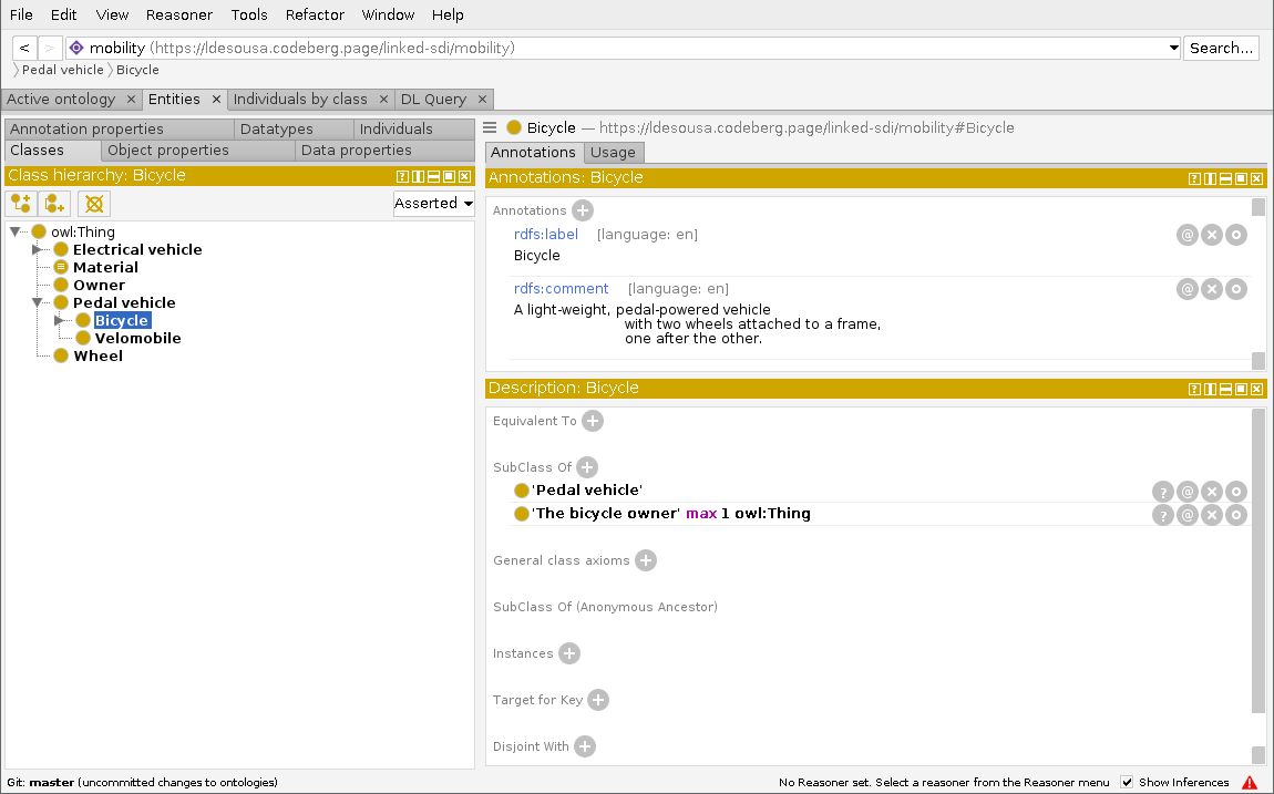
The Object properties sub-panel details exactly
those triples that associate the different classes in the ontology.
Expand the tree node owl:topObjectProperty and select one
of the properties like in Figure 8. Note the useful display of range and
domain in the Description section. As before, all triples with
the property as subject can be edited with the usual set of buttons. The
Data properties sub-panel is in all similar, as Figure
9 shows. Select the size property and inspect how the
limits to the range are portrayed. In one of the object properties click
on the edit button (o) and observe the set of data types made
available by default.
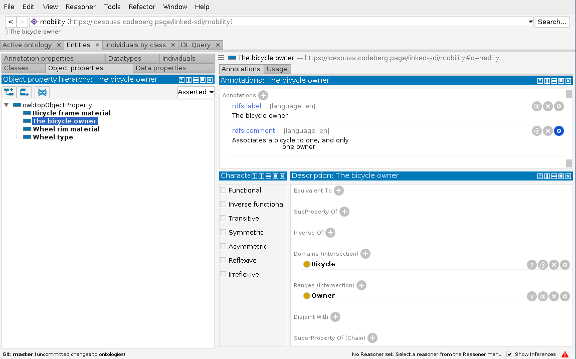
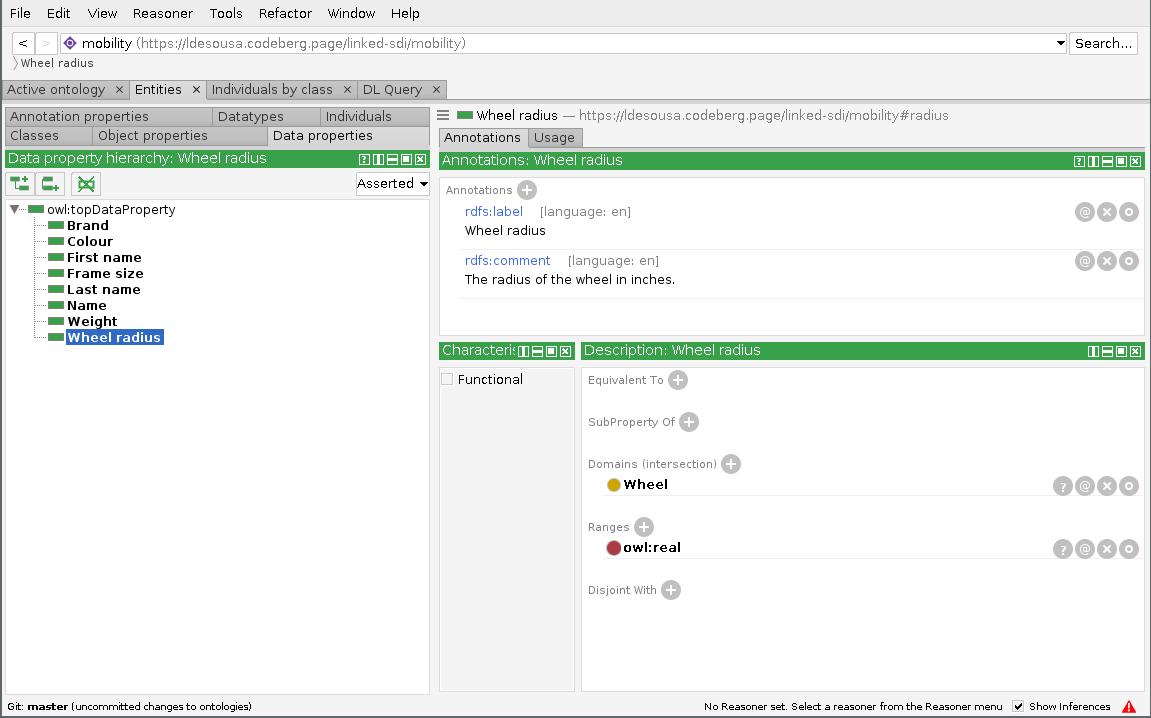
In the Individuals panel you are presented with a
list of all class instances in the ontology. In the case of Mobility
there are only the three types of frame materials (Figure 10).
Experiment adding a new material, say Bamboo, in this
panel. Make sure the new individual URI is correct and the class
Material is referenced. In ontologies with many instances
this sub-panel can be difficult to navigate, that is why the
Individuals by Class panel exists. Open it and navigate to the
Material class in the hierarchy, as Figure 11 shows.
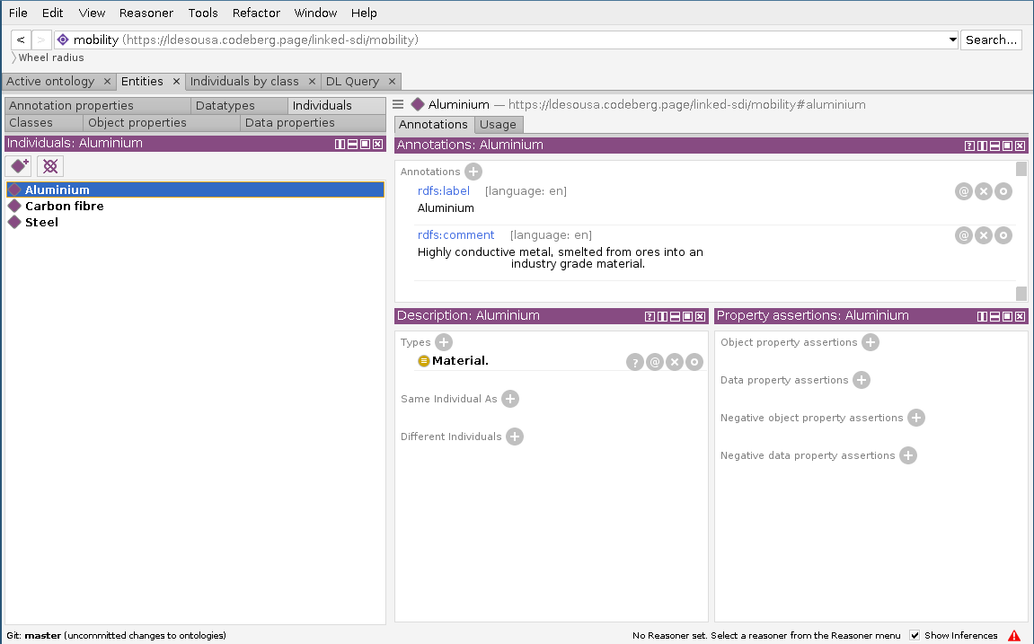
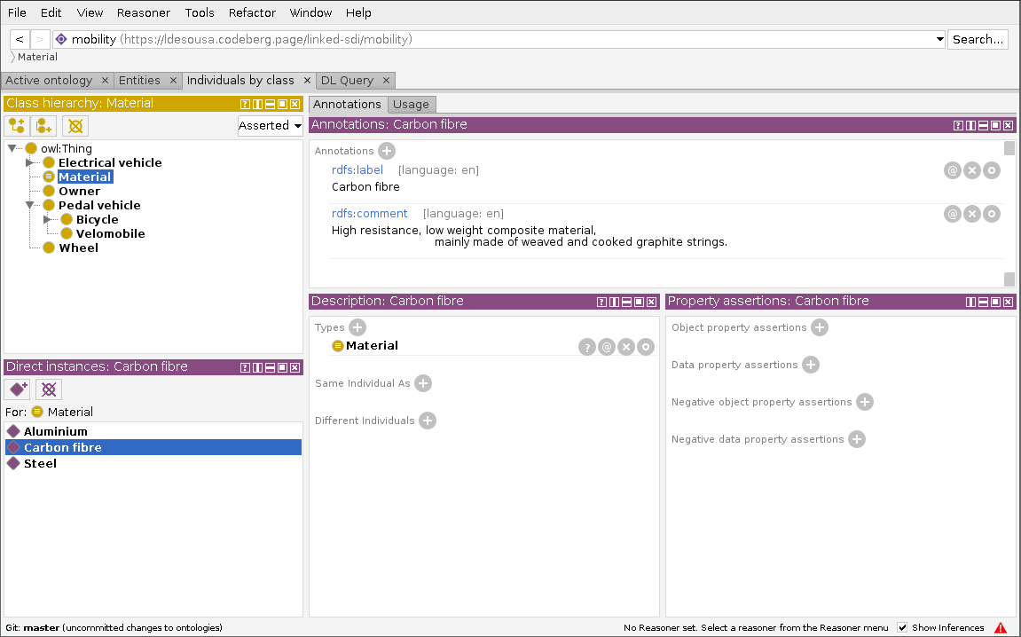
Protégé is a remarkably powerful tool, the paragraphs above only scrape the surface. However, ontology development is not the focus of this manuscript, and as geo-spatial data provider or analyst, in most cases you will use Protégé to inspect existing ontologies. With it and the knowledge you acquired on OWL in this chapter, you should be comfortable interpreting an ontology and creating knowledge graphs making use of its semantics.
3.5 Notable Web Ontologies
In practice you are unlikely to ever need to develop a new web ontology from scratch. In the vast majority of circumstances you rather use existing ontologies to encode data as knowledge graphs. In some cases perhaps extend and existing web ontology to the specifics of your data. In more than 20 years of Semantic Web many ontologies have been published that are certain to cover most, if not all, of your needs. That not being the case, you will still be using third party ontologies to represent common aspects of your data such as units of measure or geo-spatial location. The broad application of common ontologies is one of the key elements in linking Linked Data.
This section reviews a number of popular and useful ontologies, found in many knowledge graphs. Most are de facto standards, either for being recommendations of the W3C or simply for their broad adoption. To identify other ontologies, perhaps more specific to your domain, you may use a dedicated search engine such as FAIRsharing.org7. This manuscript reviews in more detail ontologies dedicated to meta-data in Chapter 9.
3.5.1 SKOS
The Simple Knowledge Organisation System (SKOS) (Miles and Bechhofer 2009) is
an ontology for the representation of vocabularies, code-lists,
thesauri, taxonomies, classification systems and similar structures of
controlled content. This ontology is centred on the Concept
class, an atomic knowledge element that although labelled in different
ways (e.g. in different languages) retains the same meaning. Concepts
are related together in a network or hierarchy.
The development of SKOS started in the very early days of the Semantic Web, pre-dating OWL itself. Within the EU funded DESIRE II project an ontology based on RDF was researched, leading also to one of the earliest proposals for query languages for the Semantic Web (Decker 1998). DESIRE II was followed by other European funded initiatives that evolved, or built upon, that early work on semantic thesauri, namely the LIMBER and SWAD-Europe projects. After 2004 the development was carried on by the W3C, eventually leading to a formal recommendation released in 2009. SKOS is widely used, and is supported by various tools that facilitate the publication of controlled content online (more on these in Chapter 8).
SKOS is remarkably simple, actually one of its strengths. At its core are five primitives:
Concept - realised by a class with the same name, represents a unit of thought, an idea, a meaning, a category or an object. Concepts are identified with URIs.
Label - data type property linking to a lexical string that annotates a concept. The same concept may be annotated in different natural languages.
Relation - a semantic association between two concepts, conveying hierarchy or simply connecting concepts in a network. Realised by object properties such as
broader,narrower, orrelated.Scheme - an aggregator class of related concepts, usually forming a hierarchy.
Note - provides further semantics or definition to a concept. Often used to associate a concept to other knowledge graphs or other external resources.
In the Mobility ontology there is a small vocabulary that can be
expressed with SKOS: the type of build material. Listing 41 exemplifies
its use, starting with an instance of the ConceptScheme
class, declaring a vocabulary and identifying its members. The
Materials class remains largely unchanged, as it is the
range of the buildMaterial object property, but it
additionally declares itself as a sub-class of Concept. The
material instances themselves declare also their nature as concepts and
use the SKOS predicates for annotations. In addition, the predicates
inScheme and topConceptOf create a small
hierarchy within the scheme.
The object properties broader and narrower do
not feature in the small example of Listing 41, but would be used to
structure further hierarchical levels. For instance a material of the
type “high-modulus carbon” could be declared as a narrower concept of
the broader “Carbon fibre”.
Listing 41: Bicycle build materials expressed with SKOS.
@prefix : <https://www.linked-sdi.com/mobility#> .
@prefix skos:  <http://www.w3.org/2004/02/skos/core#> .

materialScheme rdf:type skos:ConceptScheme ;
                skos:prefLabel
                     "Vocabulary of bicycle materials"@en;
                rdfs:label "Vocabulary of bicycle materials"@en;
                skos:hasTopConcept
                     (:aluminium :steel :carbonFibre) .

:Material rdf:type owl:Class ;
          rdfs:subClassOf skos:Concept ;
          rdfs:label "Material."@en ;
          rdfs:comment
               """ An industrial material used to build main
                   bicycle parts. """@en ;
          owl:oneOf (:aluminium :steel :carbonFibre) .

:aluminium rdf:type skos:Concept, :Material ;
           skos:inScheme :materialScheme ;
           skos:topConceptOf :materialScheme ;
           skos:prefLabel "Aluminium"@en ;
           skos:definition
                """ Highly conductive metal, smelted from ores
                    into an industry grade material."""@en .

:carbonFibre rdf:type skos:Concept, :Material ;
             skos:inScheme :materialScheme ;
             skos:topConceptOf :materialScheme ;
             skos:prefLabel "Carbon fibre"@en ;
             skos:definition
                  """ High resistance, low weight composite
                      material, mainly made of weaved and cooked
                      graphite strings."""@en .

:steel rdf:type skos:Concept, :Material ;
       skos:inScheme :materialScheme ;
       skos:topConceptOf :materialScheme ;
       skos:prefLabel "Steel"@en ;
       skos:definition
            "Alloy composed primarily by Iron and 1% to 2% Carbon."@en .
The base URI of SKOS is
http://www.w3.org/2004/02/skos/core#, usually abbreviated
to skos:. If you ever need to create or publish
vocabularies, thesauri or code-lists on the Semantic Web, you are most
advised to use SKOS. It has become a de facto standard, widely
used. A typical use case of SKOS is the extension or specilisation of
the code-lists in the INSPIRE registry 8.
3.5.2 SOSA
Over a decade ago the OGC sponsored the development of a domain model
for the interchange of observation data of natural phenomena. The result
became known as Observations and Measurements (O&M) and was also
approved as an ISO standard (Cox 2011). O&M puts forth the concept
of Observation has an action performed on a
Feature of Interest with the goal of measuring a certain
Property through a specific Procedure. More
recently, O&M made the point of departure for a web ontology
developed jointly by the OGC and W3C with similar goals, plus a further
focus on the Internet of Things (IoT). The Sensor, Observation, Sample,
and Actuator ontology (SOSA) is thus an RDF-based counterpart to O&M
(Janowicz et al.
2019).
The core concepts in the SOSA ontology are depicted in Figure 12 and can be summarised as:
Feature of Interest: a physical entity that is object of study or observation. A tree would be a feature of interest.
Property: a specific characteristic of the feature of interest that is measured. The height of a tree, or its age are properties.
Procedure: an action executed to measure the property of a feature of interest. Photographing or using a crane would be procedures to measure the height of a tree.
Unit of Measure: a well defined unit (ideally standard) on which a measurement is expressed. The eight of a tree would be expressed in metres.
Observation: a set of information identifying precisely the nature of a measurement, referring a property, a unit of measure, a procedure and/or a sensor.
Sensor: a tool or apparatus employed to conduct a measurement. A camera is the sensor used to measure a tree height through photogrametry.
Result: expresses the outcome of applying an observations on a feature of interest. It can be numerical, textual or composed. A specific tree can be assess to be 10 metres high through photogrametry.
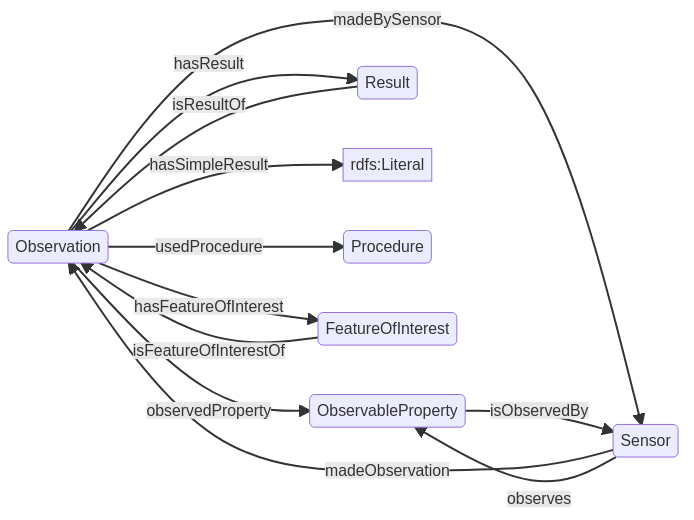
SOSA is becoming an ubiquitous ontology, starting to feature in many
knowledge graphs and other ontologies with a spatial aspect. An update
to SOSA is likely to be developed in the coming years, with the imminent
approval of Observations, Measurements & Sensors (OMS), a successor
to O&M. SOSA features in the Agriculture Information Model (AIM) and
other web ontologies to be specified in the future by the OGC. In the
turtle syntax SOSA is usually abbreviated to sosa:, with
the base URI being http://www.w3.org/ns/sosa/.
3.5.3 QUDT
The Quantities, Units, Dimensions and Types (QUDT) (QUDT.org 2011) ontology results from an effort by a group of industries in the United States towards interoperable specifications of units of measure for the scientific and engineering domains. It is composed by a unified ontological architecture on which a broad vocabulary is maintained. QUDT implements various international standards, most notably the International System of Units (ISU), thus being a foundational means for system operability. A non-for-profit organisation named QUDT.org was set up to govern the maintenance and evolution of the ontology.
QUDT is rather large, organised in various ontological modules to
facilitate their use. Two of these provide the semantic architecture
(the QUDT and Datatype ontologies), with seven additional modules
encoding the vocabularies. Table 5 digests this architecture, including
base URIs. The last element in the URI path is commonly used as
abbraviation (e.g. qudt:, datatype:).
| Content | URI |
|---|---|
| Main QUDT Ontology | http://qudt.org/schema/qudt |
| Datatype Ontology | http://qudt.org/schema/datatype |
| Units Vocabulary | http://qudt.org/vocab/unit |
| QuantityKinds Vocabulary | http://qudt.org/vocab/quantitykind |
| DimensionVectors Vocabulary | http://qudt.org/vocab/dimensionvector |
| Physical Constants Vocabulary | http://qudt.org/vocab/constant |
| Systems of Units Vocabulary | http://qudt.org/vocab/sou |
| Systems of Quantity Kinds Vocabulary | http://qudt.org/vocab/soqk |
QUDT is one of the most useful ontologies for the Semantic Web and
the internet at large, relevant to the provision of almost every
numerical datum. It is often used together with SOSA to express units
associated with observations. Even more than SOSA, you are unlikely to
ever need to specialise QUDT, the most common use case is to use one or
more of the units it defines to add that semantic clarity to your
ontologies or knowledge graphs. Therefore the most common action is to
browse the vocabularies for the appropriate instances. As an example,
bicycle frame sizes are expressed in the ISU unit centimetre, Listing 42
shows how that information can be included in the size data
property of the Mobility ontology.
Listing 42: Unit information added to the size data property with QUDT.
@prefix : <http://www.linked-sdi.com/mobility#> .
@prefix owl: <http://www.w3.org/2002/07/owl#> .
@prefix rdf: <http://www.w3.org/1999/02/22-rdf-syntax-ns#> .
@prefix rdfs: <http://www.w3.org/2000/01/rdf-schema#> .
@prefix qudt: <http://qudt.org/schema/qudt/> .
@prefix unit: <http://qudt.org/vocab/unit/> .

:size rdf:type owl:DatatypeProperty ;
      rdfs:label "Frame size"@en ;
      rdfs:comment
           """ Distance between the bottom bracket axis and a
               perpendicular to the steering set. Measured in
               centimetres."""@en ;
      qudt:unit unit:CENTIMETER ;
      rdfs:domain  :Bicycle ;
      rdfs:range [ rdf:type rdfs:Datatype ;
                   owl:onDatatype xsd:integer ;
                   owl:withRestrictions ( [ xsd:minInclusive 40 ]
                                          [ xsd:maxInclusive 64 ]
                                        )
                 ] .
3.5.4 Friend of a Friend
Friend of a Friend (FOAF) was one of the earliest ontologies expressed in OWL and the first to capture personal relationships on the Semantic Web (Brickley and Miller 2004). It was informally developed by a group of enthusiasts, without any concrete institutional backing or hosting. An open community gathered around it, fostering development up to the final release in 2014. FOAF specifies axioms describing persons, how they relate to each other and to resources on the internet. From a personal profile described with FOAF it is possible to automatically derive information such as the set of people known to two different individuals. Early in its space and relatively lightweight, FOAF went to become an important feature of the Semantic Web, used to relate and describe people responsible or associated to web resources. FOAF would influence the ActivityPub specification of the W3C (Lemmer-Webber et al. 2018), that today underlies the Fediverse9.
Developed two decades ago, FOAF is starting to show its age in some regards, with classes and predicates reflecting a stage of the internet prior to social media and individual content creation. However, a sub-set of classes remains relevant and in use:
Agent: a thing that performs actions or creates new things.Person: sub-class ofAgentrepresenting people.Organization:sub-class ofAgentrepresenting institutions such as companies or societies.Group: sub-class ofAgentrepresenting a collection of individual agent instances that share one or more common traits. Comprises concepts such as “community”, or “informal” group.Document: anything that can be broadly identified with the general definition of “document”, be it physical of electronic.PersonalProfileDocument: sub-class ofDocumentcorresponding to a RDF document describing the author (instance ofPerson) of that same document.Image: sub-class ofDocument. Although not limited to that definition, it is mostly used to instance digital images.OnlineAccount: the provision of some on-line service by a third party to anAgentinstance.OnlineEcommerceAccount: subclass ofOnlineAccountspecialised for on-line sales of goods or services.Project: broad concept for anything fitting, formal or informal, collective or individual.
Figure 13 presents the main object properties in the FOAF ontology.
Note the direct relations to rdfs:Resource from the Agent
class and to Document from the Person class.
The base URI of this ontology is
http://xmlns.com/foaf/0.1/, usually abbreviated as
foaf:.
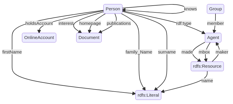
3.5.5 DBpedia
FOAF is not the only useful ontology to result from a community
effort. A similar story can be told of DBpedia, an effort to expose
common features in Wikipaedia pages as Linked Data. It is both an
ontology and a knowledge graph, the former providing semantics to the
latter. Both are under continuous update from the community, in tandem
with the evolution of Wikipaedia itself. The ontology outlines a deep
network with almost 800 classes (mostly hierarchical), complemented and
related by a collection of 3 000 properties. The number of instances in
the knowledge graph is currently more than 4.2 million. The most
instanced classes are Person, Place,
Work, Organisation and Species.
The DBpedia is automatically generated from Wikipaedia info-boxes. A
large pool of mappings from these info-boxes to the ontology provides
for the automation. These mappings are maintained publicly by the
community in a Wiki-type website10. In this Wiki
community members may also define modifications and extensions to the
ontology, to improve the mapping between Wikipedia and DBpedia.
The number of geographic locations expressed as instances of the
Place class is closing on one million. These instances do
not provide actual geographic information with coordinates, rather
triples conveying spatially relevant properties. Among the predicates
specified for this purpose are found:
countryCodemunicipalityCodealtitudenutsCodeiso31661Codeelevation
The base ontology URI is http://dbpedia.org/ontology/,
commonly abbreviated to dbo:. A dedicated web site provides
various means to navigate the DBpedia ontology, starting from the top
classes in the hierarchy and related properties11.
Meant to be explored through a SPARQL end-point. The SPARQL language is
introduced in Chapter 5.
3.5.6 Basic Geo Vocabulary
The need to represent spatial location emerged early in the development of the Semantic Web. Discussions within the W3C RDF Interest Group prompted development of a simple ontology for the purpose, eventually resulting in the Basic Geo Vocabulary (Brickley 2003). It specifies a minimal set of classes and properties to express locations with latitude, longitude and altitude in reference to the WGS84 datum ensemble. This ontology was meant to be as lightweight as possible to easily link resources expressed with other early ontologies such as FOAF. The goal was for instance to find all persons related to a same location.
The ontology specifies solely two classes:
SpatialThing: anything with spatial extent, i.e. size, shape, or position, e.g. people, places, bowling balls, as well as abstract areas like cubes.Point: a sub-class ofSpatialThing, typically described using a coordinate system relative to Earth, such as WGS84.
A set of data type properties are defined with
SpatialThing as domain:
lat_long: A comma-separated representation of a latitude, longitude coordinate.long: The WGS84 longitude of a SpatialThing (decimal degrees).latitude: The WGS84 latitude of a SpatialThing (decimal degrees).alt: The WGS84 altitude of a SpatialThing (decimal meters above the local reference ellipsoid).
The range of these properties is rdfs:string, in decimal
metres for alt and decimal degrees for the remainder.
Listing 43 provides a simple example of usage.
Additionally, a single object property is defined with
SpatialThing as range: location. It relates
any kind of resource to a spatial object (of any kind), expressing the
spatial location of the resource. This property is meant as the main
gateway to link instances on a spatial basis from different knowledge
graphs (possibly using distinct ontologies).
The base URI of this ontology is
http://www.w3.org/2003/01/geo/wgs84_pos#, commonly
abbreviated to geo:. However, you are unlikely to ever user
this ontology as it was superseeded in 2013 with the release of
GeoSPARQL (the main course in the second half of this manuscript). These
days the abbreviation geo: is mostly used relative to
GeoSPARQL instead (check the prefixes section in any case).
Listing 43: Unit information added to the size data property with QUDT.
@prefix rdf: <http://www.w3.org/1999/02/22-rdf-syntax-ns#> .
@prefix geo: <http://www.w3.org/2003/01/geo/wgs84_pos#> .
@prefix : <http://my.example.com#> .

:myPoint rdf:type geo:Point ;
         geo:lat "55.701" ;
         geo:long "12.552" .
3.6 The Cyclists knowledge graph
Something more is necessary before this manuscript can follow on to
other topics. Having defined an ontology, it would be interesting to put
it to use, creating suitable triples. That is the role of the “Cyclists”
knowledge graph, accessible on-line at the URI
https://www.linked-sdi.com/cyclists# and also reproduced in
Annex B. It declares a number of imaginary people, plus the author, and
relates them to a set of bicycles. For each bicycle a set of simple
characteristics are given with axioms from the “Mobility” ontology. Take
some time to pore through the knowledge graph. Is it entirely
understandable? Would you choose to encode the same information in a
different way?
4 Triple Stores
The knowledge graphs this book has shown you so far are fairly small, with triples counted in the dozens. As you may imagine, most knowledge graphs are much larger. A knowledge graph reporting addresses and geo-spatial features for the dwellings of a small town easily reaches the thousands of triples. Costumer data for a nation-wide service or company rapidly reaches the realm of milliards. Naturally, such real-life sized knowledge graphs can not possibly be published as simple documents in a web server. Just as relational data can be stored in relational database storage systems, RDF can be stored by a type of programme named Triple Store. These programmes not only provide efficient RDF storage/retrieval, they also make available an essential feature of the Semantic Web: the SPARQL end-point. This is the data search service usable by both humans and machines, powered by the human discourse mimicking query language introduced in Chapter 5.
At present there are three reference triple stores supporting geo-spatial RDF: (i) Openlink Virtuoso, (ii) Apache Fuseki, and (iii) Eclipse RDF4J. This chapter introduces the first two, with install and basic interaction instructions, covering both the C and Java programming worlds. In the subsequent chapters of this manuscript it will be important to have one of these triple stores functioning on your system to test and experiment with the various knowledge graphs presented.
4.1 Virtuoso
4.1.1 Overview
Virtuoso can perhaps be best described as the Swiss knife of data storage. It aims to support all major paradigms of data back-end: be a relational database management system (RDBMS), an object-relational database, and store XML, full-text and other file-based formats. Virtuoso further provides functionality as a web application server and file server. And yes, it also supports RDF, functioning as a triple-store. Moreover, it implements GeoSPARQL, making it a geo-spatial triple-store.
Virtuoso is written with the C programming language and is designed to run as a multi-threaded server. These aspects make it a fast and lightweight server, requiring few resources, and easy to manage in containerised environments. It can function both with physical file storage as well as in memory storage mode for performance purposes. C also makes it cross-platform: 32 and 64 bit architectures; Linux, Unix, Windows and macOS.
The origins of Virtuoso root back to the Computer Science scene of the late 1980s in Finland, in a time when various data storage tools were being developed around the Lisp and Prolog programming languages. Out of this community various reference RDBMS technologies emerged in the 1990s: MySQL, InnoDB, Solid and Kubl. In 1998 OpenLink, a data access middleware company, acquired Kubl, from that merger giving shape to the all-encompassing Virtuoso project. Virtuoso would develop in parallel (or tandem) with the Semantic Web, bridging much of the influence from the Finish community on the standards and recommendations of the W3C.
Virtuoso is much more than a triple-store, providing functionalities regarding data publication that can be very useful to data providers in the Semantic Web. These functionalities coupled with its performance and lightweight make of Virtuoso an obvious choice as the backbone of geo-spatial linked data infrastructure.
4.1.2 Setting up
OpenLink maintains its own repository of containerised images at DockerHub (O. Software 2021). These images make the deployment of Virtuoso fairly convenient, both for development, testing or production environments. The company publishes the most recent versions, and advises users to prefer this repository over others not related to the company. This section focus on the set-up of a containerised Virtuoso instance for development with the Docker technology. The specifics of a production environment deployment are beyond the scope of this text, although the information here should provide good insight.
Assuming you have Docker installed on your system, the first thing to do is fetch the Docker image from the upstream repository (Listing 44).
Listing 44: Pulling latest image for Virtuoso 7
docker pull openlink/virtuoso-opensource-7Next you need to create a folder for Virtuoso to store its internal
storage files. It is advisable not to create this folder in the system
volume. In a development environment it can reside in the user area. In
production it probably sits better on an external volume (possibly with
back up). In development a two folder structure is recommended, a parent
folder in which set-up files reside and a sub-folder for the actual
database (e.g. mkdir -p virtuoso/data).
To start a new container from the Virtuoso image, a few parameters must be declared:
- the ports exposed (one for the interactive service and another for the web interface);
- the database volume;
- the administrator password.
All these parameters can be passed through the command line to Docker
with the run command. However, a better option is to create
a configuration file to facilitate re-use. Docker Compose (Inc. 2021) is a
convenient tool for this purpose, especially since it is possible you
will run other applications with Virtuoso (if not already, probably
later). Listing 45 provides an example for a
docker-compose.yml file. Virtuoso uses ports 1111 and 8890
by default, since these are unlikely to clash with other applications
they can be mapped ipsis verbis. Then the database
volume is mapped to the folder created in the host system. And finally
the environment variable DBA_PASSWORD is set.
Listing 45: Example Compose set-up file for Virtuoso
version: '3.3'

services:
  virtuoso:
    image: openlink/virtuoso-opensource-7:latest

    container_name: virt-db

    ports:
      - 1111:1111
      - 8890:8890

    volumes:
      - ./data:/database

    environment:
      - DBA_PASSWORD=secret
You may at last start the new container with the command in Listing
46. To make sure everything went fine point your browser to
http://localhost:8890, a welcome page should be
displayed.
Listing 46: Starting a new Virtuoso container with docker-compose
docker compose up --build --detach4.1.2.1 Add the database path to
virtuoso.ini
For security reasons this Virtuoso image is set up with a high level of constraints on data load. By default it does not provide an expedient way to load knowledge graphs. Virtuoso requires the explicit declaration of a set of folders from which data load is allowed.
In the Virtuoso database folder (data in the example
above) you will find a file named virtuoso.ini where this
setting can be modified. Open it with your favourite file editor and
search for the parameter DirsAllowed. These folder paths
refer to the internal tree of the container, therefore, to be accessible
from the host system an additional folder should match one of the
volumes declared in the docker-compose.yml file. In
development and testing environments you can use the
database folder directly (as Listing 47 exemplifies). In
production it might be wiser to set up a specific volume for this
purpose in the docker-compose.yml configuration.
Listing 47: Setting the database folder as an allowed source of external data in virtuoso.ini.
DirsAllowed = ., ../vad, /usr/share/proj, /databaseOn a Linux system the files inside the Virtuoso database
folder are owned by the system administrator (root). Thus you likely
need to authenticate as administrator to modify the
virtuoso.ini file. After modifying this file Virtuoso might
not immediately assume the set-up changes. In such case you need to
restart the container, for instance with the docker restart
command.
4.1.3 Basic interaction
4.1.3.1 Start a command line session in the container
As many other data storage systems, Virtuoso provides a client tool
for basic interaction through the command line. While not the most
expressive, these tools are powerful and useful, either to interact with
a production server or to process data in bulk. This tool is named
isql and as its name implies, was originally meant for the
SQL language. However it also exposes many additional functions and can
also interpret the SPARQL language (Chapter 5).
The Virtuoso docker image already includes the isql
client, thus there is no need to install it on the host system. In
effect isql is run by the container itself. A new session
can be initiated with the docker exec command, passing to
isql the interactive port. If you did not change the
defaults its number will be 1111. Listing 48 provides an
example, with the -i parameter used additionally to
identify the running Virtuoso container.
Listing 48: Starting a new interactive session with isql within the Virtuoso docker container.
docker exec -i my_virtdb isql 11114.1.3.2 Load a Turtle file with a graph URI
With the software set up and ready to use there isn’t yet much you
can do, since no data has been loaded into the store. Data load is
likely the first action you will wish to do in a triple store like
Virtuoso. The most straightforward option is to use one of the built-in
functions to load a knowledge graph. One of these functions is
DB.DBA.TTLP_MT, which is able to load Turtle, N-Quad or
N-Triple files into the triple store.
The arguments taken by DB.DBA.TTLP_MT are the following
in this same order:
- strg: path to the file to load;
- base: base URI used to resolve all relative URIs in the input file;
- graph: general URI used to identify all the triples in the knowledge graph;
- flags: bit mask allowing certain syntax errors in the source file; 0 by default, i.e. no errors allowed;
- log_mode: type of messages recorded in the Virtuoso log, from 0 for low (by default) to 2 for high;
- threads: number of CPU threads to use; transactional: 0 for off (default) or 1 for on.
In most circumstances only the first three arguments are necessary.
The base URI can be an empty string if there are no relative URIs in the
input file. It is useful if the name of the graph matches the base URI
of the triples, i.e. the abbreviation declared with the
@prefix keyword in a Turtle file. For the knowledge graph
created in Section 3.6 with the string
https://www.linked-sdi.com/cyclists# would be an
appropriate choice. The path to the input file refers to the internal
tree structure of the container. If you use a set-up similar to that
exemplified above, you can simply copy the input file to the host folder
matching the dataset volume. Finally,
DB.DBA.TTLP_MT requires the path string to be transformed
with another function: file_to_string_output. Listing 49
presents an example with the Cyclists graph. If you have not done so
yet, give it a try.
Listing 49: Loading a knowledge graph to Virtuoso with `DB.DBA.TTLP_MT`.
DB.DBA.TTLP_MT (
    file_to_string_output('/database/Cyclists.ttl'), '',
    'https://www.linked-sdi.com/cyclists#'
);
4.1.3.3 Bulk load from a folder
In case there is a large number of files to process, for instance if
the graph is very large, or you need to import a large number or graphs,
applying the DB.DBA.TTLP_MT function to each file might be
too cumbersome. In alternative it is possible to load the full contents
of a folder in the hard drive all at once with the ld_dir
function. This function takes only three arguments: (i) path to the
folder, (ii) matching file pattern and (iii) graph URI. Listing 50 shows
an example. In effect ld_dir only instructs Virtuoso on the
location of the resources to load. To make sure all the desired
resources have been correctly identified by the ld_dir
function you may query the DB.DBA.load_list table in the
Virtuoso internal relational database. The actual data load only starts
once the rdf_loader_run() function is called. Then the
loading process runs in the background and can be verified with the
checkpoint instruction (in case it is lengthy). One of the
advantages of ld_dir is the vast range of file formats it
is able to parse. It includes:
- Turtle (
.ttl) - N-Triples (
.nt) - XML (
.xml,.rdf) - N-Quads (
.nq,.n4)
Listing 50: Loading all the knowledge graphs from a folder with `ld_dir`.
ld_dir(
    '/database/my-graph/', '*.ttl',
    'http://www.example.org/POI#'
);
SELECT * FROM DB.DBA.load_list;
rdf_loader_run();
checkpoint;
4.1.3.4 List existing knowledge graphs
After loading one or more graphs it is important to check the status
of the triple store, even if the process went without errors. The
isql tool is able to interpret SPARQL queries, with which
it is possible to conduct some basic inspection on existing graphs.
Listing 51 provides a simple example listing all the graphs stored by
Virtuoso.
Listing 51: List existing knowledge graphs in a Virtuoso triple store with a SPARQL query.
SPARQL
SELECT DISTINCT ?g
 WHERE {GRAPH ?g {?s ?p ?o}};
Note how the query in Listing 51 starts with the SPARQL
statement. This statement is not part of the SPARQL standard, it is
specific to isql, to distinguish a SPARQL query from a SQL
query. The remainder of the query is rather simple SPARQL, no need to
worry too much at this stage. You may dive into SPARQL in more detail in
Chapter 5 where you will learn to build more refined queries from the
simple example above.
4.1.3.5 Count triples in a knowledge graph
Another useful way to inspect a graph after loading is counting the
number of triples it contains. SPARQL is again a useful means to obtain
such information through isql. Listing 52 uses the
COUNT statement to count the triples in the Cyclists
knowledge graph.
Listing 52: Count number of triples in a knowledge graph in a Virtuoso triple store with a SPARQL query.
SPARQL
SELECT COUNT (?s)
  FROM <https://www.linked-sdi.com/cyclists#>
 WHERE {?s ?p ?o} ;
4.1.3.6 Remove a knowledge graph
Finally, there is always a circumstance in which it is necessary to
remove a knowledge graph from the triple store, either to replace it,
because it had errors, or simply if it became outdated. Virtuoso makes
available a specific statement for this purpose:
CLEAR GRAPH, taking as single argument the URI of the
graph. Listing 53 provides an example, where again the
SPARQL statement marks the start of the query.
Listing 53: Count number of triples in a knowledge graph in a Virtuoso triple store with a SPARQL query.
SPARQL
CLEAR GRAPH  <https://www.linked-sdi.com/cyclists#>;
4.1.3.7 Direct query output to a text file
Another useful feature, pretty much of any command line tool, is the
possibility to redirect output to a text file. This is not possible
directly from the isql prompt, however, the parameter
exec allows the user to pass a query for non-interactive
execution, returning results to the standard output. Then it is just a
matter of redirecting the standard output to a file. Listing 54 offers
an example, running isql from the Virtuoso container, with
a SPARQL query passed to the exec parameter and the output
redirected to a file named out.txt. Note also the need to
pass username and password, as this is not an interactive session.
Listing 54: Redirection of a query output to a file with isql.
docker exec -i my_virtdb isql 1111 dba secret exec="
SPARQL
PREFIX rdfs:  <http://www.w3.org/2000/01/rdf-schema#>
PREFIX sosa:  <http://www.w3.org/ns/sosa/>
SELECT DISTINCT ?obs
WHERE {
    ?obs rdfs:subClassOf sosa:Observation .
};" > out.txt
4.1.4 The Web Interface
Beyond text based interaction through port 1111, Virtuoso makes
available a rich web interface through port 8890. It is also through
this port that Virtuoso is meant to be queried from external clients,
through the HTTP protocol. In particular, Virtuoso provides access to
the triple store through SPARQL queries at the address
http://your-server:8890/spaqrl. This path to SPARQL
interaction over HTTP is commonly known as “SPARQL endpoint”.
This section offers a brief overview of the administration
functionalities available through the web interface regarding RDF. If
you point your web browser to http://localhost:8890 you
will be greeted with a welcome page as Figure 14 shows. This page is a
gateway to various aspects of Virtuoso, such as the SPARQL endpoint, the
Faceted browser (to be explored in Chapter 8.1), tutorials, overall
documentation plus, a few links back to the OpenLink website. The
administration aspect is called “Conductor”, which you can access by
clicking the topmost button in the left side menu.
The first page in Conductor gives an overview of its different goals. At the top a series of tabs provides access to the different functions performed by Virtuoso, from data store to web services. In this manuscript the focus is solely on Linked Data, all the other aspects are beyond its scope. Before anything else you need to log on to Conductor, use the same credentials you set up in the docker compose set up (Listing 45).
Upon logging in, click on the Linked Data tab, Conductor
then brings you to a graphical interface to the SPARQL endpoint, as
Figure 16 shows. A few sub-tabs are now also in display, leading to
different administrative functions for RDF knowledge graphs. Give a try
to the SPARQL interface, copy one of the queries in Listing 52 or
Listing 51 into the Query text box, remove the
SPARQL prefix in the first line and the last ;
character. Leave the Graph URI text box empty and press the
Execute button.
Click now on the Quad Store Upload12
sub-tab, Conductor takes you to yet another mechanism to load a
knowledge graph into the triple store. With the radio buttons you can
chose whether to load the graph from a file or from a URL. In the latter
case Conductor loads all the triples it can fetch from that location.
Experiment loading the knowledge graph for the VCard ontology, insert
the URI http://www.w3.org/2006/vcard/ns# in the
Resource URL text box and add the same to the Named Graph
IRI text box, then press the Upload button. It is
important to provide the URI to name the graph, it facilitates querying
later on. Otherwise the loaded triples end up in the default knowledge
graph (http://localhost:8890/DAV/). Chapter 9 provides the
details on VCard, and its role in meta-data creation and
publication.
Click now on the Graphs sub-tab to access the Conductor knowledge graph administration area. Yet another set of sub-tabs unfolds, most related to user access control. These administration details are not explained here (although keep in mind you can fine tune who is able to access each knowledge graph), the relevant bit is the new Graphs sub-tab. It presents a list of the knowledge graphs currently loaded in the triple store (Figure 18). Here you can remove or rename one of these graphs, clicking the links on the righthand side. Try removing the VCard knowledge graph, and if successful go back to the Quad Store Upload sub-tab and load it again.
The web interface provides additional information for each knowledge graph in the form of summary statistics. In the Graphs tab copy the URI of one of the knowledge graphs, then open the Statistics sub-tab. Insert the URI in the Graph IRI field and click Generate. The output is itself a small RDF document displayed in the Turtle language (Figure 19). It informs on the number of triples, distinct subject and objects in the graph. Figure 19 shows statistics for an ontology (OWL) itself, thus the extra information on the number of classes and properties.
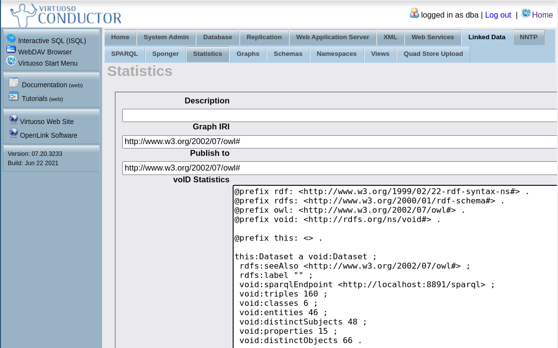
This has been a very brief introduction to Virtuoso, the software is far broader in the number of features and services it can provide. This manuscript will later return to Virtuoso to explore some of its extra data services that complement the SPARQL end-point.
4.2 Apache Jena Fuseki
The short term “Fuseki” is used in this book referring to the full software complex, but in reality two different products are at play:
Apache Jena: a toolbox for the manipulation and analysis of knowledge graphs. Meant to be used from the command line.
Apache Jena Fuseki: a triple store engine deployable to a Java web server. It provides a web based graphical user interface to manage and query knowledge graphs.
This choice of naming can be confusing, especially since the Jena toolbox is not that useful without the Fuseki triple store. In reverse, the triple store can be deployed and used stand-alone, at the loss of automation (particularly concerning data load).
Fuseki also provides a logical container for knowledge graphs, which can be seen as a super-structure above the latter. It is called the dataset, essentially grouping a set of knowledge graphs. Fuseki creates an independent SPARQL endpoint for each dataset, each with its own URL. This means a query run on a dataset will not directly consider graphs gathered in a different dataset. Keep that in mind in the set-up sections below.
Compared to Virtuoso, Fuseki presents itself as a much leaner piece of software, with a considerably smaller set of functionalities. On the one hand it is a more approachable programme, with a shallower learning curve. On the other it can become limiting in more complex contexts. And leaner does not mean lighter, as Fuseki can be more demanding on resources. More on this towards the end of this section.
4.2.1 Download and set up
The first task is to obtain the software from the Apache Foundation. One of the advantages of being a Java programme is not needing to be installed. However, you will need to have an up-to-date Java Runtime Environment installed on your system. You can access the latest Fuseki releases from the download website 13. You must obtain the compressed binaries for both programmes and expand them into some convenient place in your system, as Listing 55 shows.
Listing 55: Downloading and expanding the Jena and Fuseki binaries.
wget https://dlcdn.apache.org/jena/binaries/apache-jena-fuseki-4.6.1.zip

wget https://dlcdn.apache.org/jena/binaries/apache-jena-4.6.1.zip

unzip apache-jena-fuseki-4.6.1.zip

unzip apache-jena-4.6.1.zip
Fuseki is ready to run, but first you need to create at least one
folder to host a dataset. Fuseki hosts datasets in the
run/databases folder, the best place to create a new
sub-folder to host the dataset. The fuseki-server script
starts the server itself, requiring at least three arguments:
the location of the default dataset (passed with the
--locflag);the port on which the server should listen (passed with the
--port, flag);a simple path naming the default dataset.
In Listing 56 an example is given starting up Fuseki on port 3031 with a dataset named “/default”. Note the location path is the same created in Listing 55.
Listing 56: Starting Fuseki on port 3031 with a default dataset.
cd apache-jena-fuseki-4.6.1

mkdir run/databases/default

./fuseki-server --loc=./run/databases/default --port 3031 --update /default
4.2.2 Command line interaction
With the server up and running, you can start performing simple tasks
such as loading additional knowledge graphs to the triple store. Before
anything else, it is useful to add the Jena binary folder to the system
(or user) path. The relevant folder is
apache-jena-4.6.1/bin (if you obtained a different version
the number will be different). Adding a folder to the system path is
usually a simple operation, but since it differs from system to system
it is left as exercise.
4.2.2.1 Load data
The Jena tool to bulk load knowledge graphs is
tdb1.xloader. It can be used by simply providing a path to
the source knowledge graph and a second in which to store the imported
triples. tdb1.xloader will always create a new dataset into
which the knowledge graph is imported. Therefore you need to create a
new dataset folder, as Listing 57 exemplifies.
Listing 57: Importing a knowledge graph into a new dataset with `tdb1.xloader`.
mkdir run/databases/my-graph

tdb1.xloader --loc ./run/databases/my-dataset ~/graphs/my-graph.ttl
In case you wish to load the knowledge graph into an existing
dataset, there is the tdbloader tool in alternative. Simply
provide the path to the dataset in the run/databases
folder, using the --loc parameter, similarly to
tdb1.xloader. Both of these, and other loading tools, are
able to interpret the common RDF file formats such as RDF/XML, N-Triples
and Turtle.
4.2.2.2 SPARQL queries
Since it lacks an interactive command line environment, querying the
Fuseki triple store must also be made with the help of a specialised
tool. Its name is tdbquery and functions by reading a file
with the SPAQRL query to execute and then dumping its results to the
command line. The --loc parameter is used to identify the
dataset against which the query is executed, whereas the
--file parameter indicates the path to the query file
(Listing 58).
Listing 58: Execting a SPARQL query against an existing dataset with `tdbquery`.
tdbquery --loc run/databases/my-dataset --file ./returnTriples.ttl This particular tool executes directly on the assets stored in the
file system, independently of the triple store itself. Thefore it
completes even if Fuseki is not running. Other parameters are made
available by tdbquery that may come handy:
--time: report the time it takes to execute the query;--results: select the output format, to choose between XML, JSON, CSV, TSV or RDF;--base: provide the base URI of the query.
4.2.2.3 Obtain statistics
Simple statistics can be obtained with the tdbstats
tool. It reports the overall number of triples in a given database and
the number of triples by class. By default tdbstats applies
to the full triple store, but it can zoom on a single knowledge graph
using the --graph parameter.
Listing 59: Obtaining statistics for a dataset with `tdbstats`.
tdbstats --loc run/databases/my-dataset4.2.2.4 Retrieve a serialised knowledge graph
A dataset can be serialised with the tdb2.tdbdump tool.
This action is also informally known as “dump”, hence the name.
tdb2.tdfdump only acts on the full dataset and prompts the
output to the command line itself. As this is unlikely to be useful, you
can simply redirect the output to a file, as Listing 60 shows.
Listing 60: Serialising a dataset with `tdb2.tdbdump`.
tdb2.tdbdump --loc run/databases/my-dataset > my-dataset.nqWith the --output parameter you can specify the output
format. However this must be a quad format, i.e. identifying the
knowledge graph for each triple. By default tdb2.tdbdump
produces outputs in the N-Quads format (the extension of N-Triples to
quads). With the parametrisation --output=Trig you can
obtain a Turtle-like format. If the triples in a dataset do not identify
a knowledge graph, this output will in practice be Turtle. Also worth
noting that with the --compress parameter,
tdb2.tdbdump compresses the output with the gzip algorithm.
Useful for large datasets.
4.2.2.5 Quick reference for Jena tools
In its 4.6.1 version Jena includes a total of fifty different tools. An exhaustive review of each would be beyond the goals of this document, since their usefulness varies in the context of Linked Data infrastructures. This section briefly highlights a few that complement the more fundamental tools detailed above.
riot: the Jena Swiss Army knive. Its primary purpose is to parse RDF, but can do much more. Among its functions are: RDFS inferencing (--rdfsparameter), triples counting (--cont), serialisations conversion, syntax validation, datasets concatenatation. Assumes the input to be in the N-Triples format, but accepts others trough the--syntaxparameter.turtle,ntriples,nquads,trig,rdfxml: specialised versions ofriotthat dispense the--syntaxparameter.arqandsparql: executes a query stored in a file (astdbquery) against a serialised knowledge graph or dataset (the latter encoded in a quad format).qparse: parses a query. It reports errors if found and outputs a human-readable version of the query.uparse: operates asqparsebut for update requests.rsparql: sends a local query to a SPARQL endpoint specified with a URL. Provides the same choice of output formats asarq.rupdate: sends a local update query to a SPARQL endpoint specified with a URL.
4.2.3 Setting up a containerised service
Apache publishes Docker containerisation configurations for the most recent Fuseki releases. But these are available only from the Maven web site, they are not available as images from a web site like DockerHub. There are in fact many Jena and Fuseki images available at DockerHub but none are official and in most cases do not present a reliable packaging of the software.
4.2.3.1 Building from the official configuration
You must access the Fuseki Docker repository 14 with a web browser and manually select which version to download (the latest is recommended, 4.6.1 at the time of writing). Then download and unpack it, as Listing lst. 61 exemplifies.
Listing 61: Obtaining the latest Fuseki containerisation assets.
wget https://repo1.maven.org/maven2/org/apache/jena/jena-fuseki-docker/4.6.1/jena-fuseki-docker-4.6.1.zip

unzip jena-fuseki-docker-4.6.1.zip

rm jena-fuseki-docker-4.6.1.zip

mv jena-fuseki-docker-4.6.1 fuseki

cd fuseki
In the new fuseki folder you thus find the files
Dockerfile and docker-compose ready to build a
local container. Have a look at the docker-compose file, it
is setting two volumes, one for the service logs and another named
databases. The latter is where the actual knowledge graphs
are stored, with a map to the host system guaranteeing persistence.
Before building the container you must first create these two folders in
your system. Issuing the command docker-compose build you
can finally build a local container. Next you will likely wish to load
data to be served, for which you use a Jena tool like
tdb2.tdbloader. Listing 62 shows an example, creating a new
folders for the logs and default dataset, loading a knowledge graph and
then starting the container with the docker-compose run
command. Note how the default dataset location is passed with the
--loc parameter. The --tdb2 parameter informs
this to be a persistent instance, with datasets stored in the file
system. By adding the --update parameter Fuseki runs in
update mode, i.e., changes to knowledge graphs are persisted in the file
system.
Listing 62: Running the Fuseki container with a persistent dataset.
mkdir logs

mkdir -p databases/my-dataset

tdb2.tdbloader --loc databases/my-dataset my-dataset.ttl

docker-compose run --rm --name MyServer --service-ports fuseki --tdb2 --update --loc databases/my-dataset /ds
4.2.3.2 Java Memory management
Java is a great programming language semantically and syntathically, but is also a garbage collected language. Without going into much detail, this means Java programmes have different requirements regarding memory management. A Fuseki set up lacking memory limits can easily consume an expected amount of memory. In containerised environments this will rapidly become a problem, as the host system usually kills any process reaching the limits of allocated memory.
The JAVA_OPTIONS environment variable passed to Docker
in Listing 63 exemplifies how to set the limit of memory allocated to
the Java heap. A simple solution for a development environment. Further
details on the setup of a Java programme in a memory constrained
environment are outside the scope of this document. Memory management is
a crucial aspect when deploying a Fuseki instance to a production
environment, and can be somewhat more intricate. In case you do not
master the set up of the Java virtual machine in containerised
environments, it is better to recur to someone seasoned on the matter (a
systems administrator or “devops” technician). Also note that parameters
passed to the Java virtual machine may differ accross platforms.
Listing 63: Runng the Fuseki container with limits to the Java heap.
docker-compose run --service-ports --rm -e JAVA_OPTIONS="-Xmx1048m -Xms1048m" --name MyServer fuseki --tdb2 --loc databases/my-dataset /ds4.2.4 Graphical User Interface
With the server running, directly on the system or with a container,
you can access the graphical user interface by directing a web browser
to the right port, e.g. http://localhost:3031. Fuseki shows
a welcome page (Figure 20) listing the existing datasets, showing the
status of the server and providing entry points to various management
web pages.
Note that Fuseki does not impose by itself any kind of user filtering. There is no authentication mechanism built in. This can instead be set up with a web server, otherwise all management actions are available to whomever gains access to the Fuseki instance. It is therefore important to consider whether Fuseki should run in read/write mode when starting up the server.
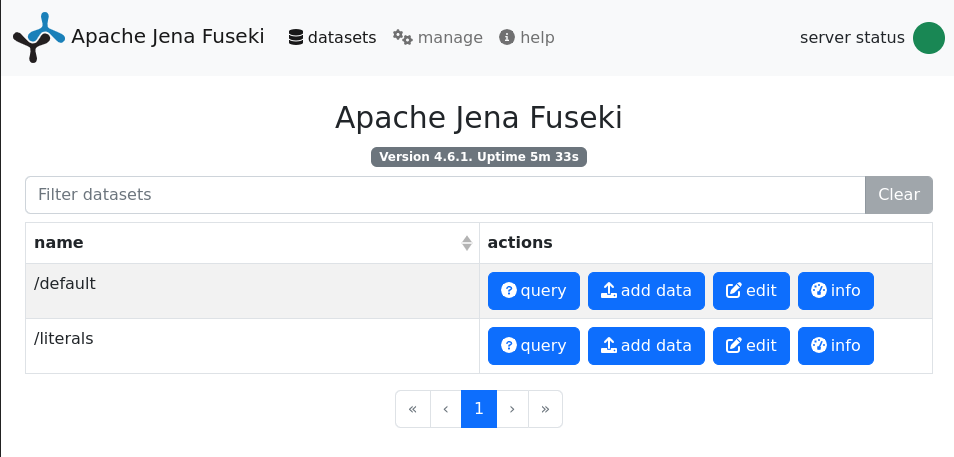
The manage link in the top bar takes you to another list of datasets, but with a broader range of actions (Figure 21). As a triple store administrator, this web page is the most useful dashboard.
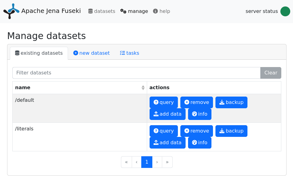
Is is also from the manage web page that you can access the form to create new datasets. Click on the new dataset tab to see its contents (Figure 22). You just need to provide a name for the new dataset and indicate whether it should be persistent (i.e. stored on the file system) or stored in memory. The latter option is lighter on resources and faster, but all its contents are discarded when the server shuts down or restarts.
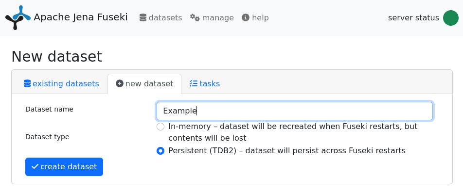
From the manage web page it is also possible to initiate the process to upload a knowledge graph into an existing dataset. Clicking on the blue button “add data” brings you to a new form for that purpose (Figure 23). The upload form has only two inputs: the knowledge graph name, a URI, and a RDF file. The latter can be selected by clicking on the green button “+ select files”. The blue button “upload all” completes the task. As the button name implies, more than one RDF file can be uploaded at a time in this form.
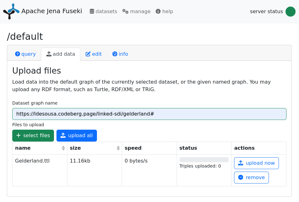
Either by returning to the manage page or by using the tabs that appear in the add data form you may access the edit form (Figure 24). At the top of the form the list of knowledge graphs assigned to the current dataset is displayed. By clicking on one of them a text edition box comes up with the contents of the graph. This is a high quality, Turtle encoded, version of the graph that you can edit directly. This is not that advisable, it is easy to make mistakes this way. However, this form provides an easy view into the details of the knowledge graph.
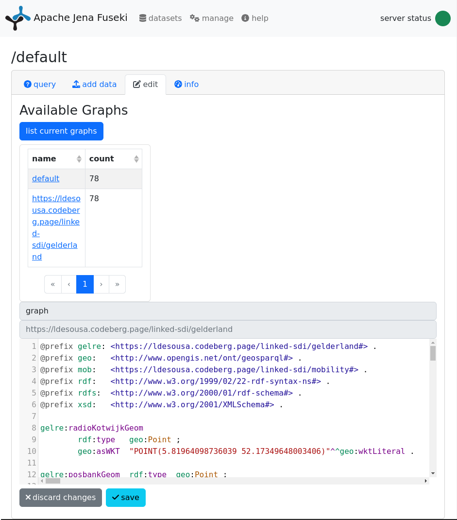
Again using the tabs, or from the manage page, you can access the info page. It provides statistics on the ensemble of knowledge graphs and also on the requests processed by Fuseki against the dataset (Figure 25). These statistics are broken down by the different end-points automatically set in place by Fuseki for each dataset. By clicking on the blue button count triples in all graphs you can get a report on the number of triples in each knowledge graph and in the dataset as a whole.
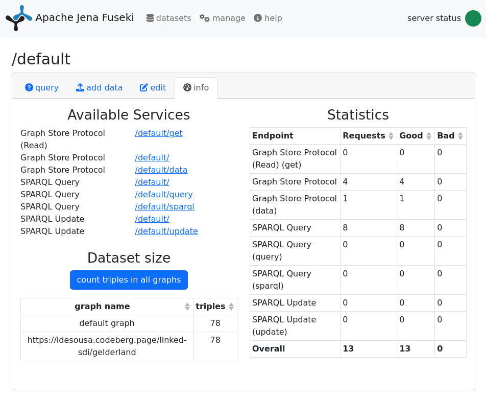
The final page to visit is the SPARQL query form, also accessible from the manage page or through the tabs (Figure 26). This might be the form on which you will spend most time and it is pretty straightforward. Type your query in the text box and on the click on the play button. Some example queries are available to get you started, as so some shortcuts to add URI abbreviations. It is also possible to apply human-friendly HTML formatting to the query output.
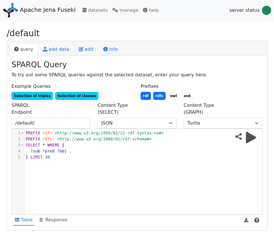
5 The SPARQL query language
5.1 Introduction
So far this book has went through the structuring, encoding and storage of data as RDF triples. Early on, directly opening RDF files in a text editor or Protègè is enough to understand a RDF graph. But it does not take long before a larger graph renders that kind of manual activity impractical. If a certain graph results in a Turtle file of several MB, is it still usable? The answer to this question is two-fold: an RDF graph that large requires dedicated storage (tackled in Chapter 4) and more sophisticated search capabilities to analyse and synthesise.
The SPARQL Protocol and RDF Query Language (SPARQL is a recursive acronym) is the second half of the answer above. It was first adopted by the W3C in 2008 (Prud’hommeaux and Seaborne 2008) and amended in 2013 (SPARQL 1.1) (Harris and Seaborne 2013). SPARQL provides the syntax to query a RDF source, laying out in normalised terms questions that could otherwise be expressed in natural language. For instance, considering again the mobility example: who owns a city bike? Which is the lightest bicycle? Which build material is most common? Etc.
SPARQL resembles the Simple Query Language (SQL) not only in name, it is very much inspired on the latter. Like SQL, SPARQL translates what are essentially set theory axioms into something very close to natural language. Segmenting a set with a logic condition, joining sets, applying a function to a set or sub-set, formally this is what these languages do. Therefore much of the SPARQL syntax is similar to SQL. Readers with an understanding of the latter might find their way through these pages easier. However RDF concerns triples, thus there are relevant differences in query construction and query result that must be well understood.
5.2 Essential SPARQL
5.2.1 Basic searches for properties
The simplest query you can make against an RDF graph is to request
the set of elements that fulfil one or more criteria. In natural
language these are questions like “Who owns a bicycle?”, “Which bicycles
are made of steel?” or “Which is the lightest bicycle?”. These questions
share a common pattern, first the what: “who”, “which
bicycle(s)”, and then a criterion: “owns a bicycle”, “is made of steel”,
“is the lightest”. SPARQL mimics this structure with a two part
structure: the SELECT clause for the what and the
WHERE clause for the criteria.
The SELECT clause lists the elements expected in the
result. These are preceded by a question mark (?) and must
also feature within the WHERE clause. The
WHERE clause encloses a set of triples within curly
brackets ({ and }). The triples in the
WHERE follow a syntax identical to Turtle, with its
elements separated by a space and terminated by a full stop. Each triple
represents a condition or criterion that must be satisfied by a triple
to be selected. The elements that are the target of search, or those
that are unknown are preceded by a question mark too. For instance, the
question “Who owns a bicycle?” is translated into the SPARQL statement
in Listing 64.
Listing 64: A simple `SELECT` query with a single match criterion.
SELECT ?owner
WHERE { ?bicycle <https://www.linked-sdi.com/mobility#ownedBy> ?owner }
This query translates into a search for all the triples with the
https://www.linked-sdi.com/mobility#ownedBy predicate.
Since both the object and the subject are unknown (with the question
mark) no restrictions are applied to those. The subjects in the triples
matching the criteria are then returned as the result.
5.2.1.1 URI Abbreviations
As with Turtle, it is possible to abbreviate URIs to obtain easier to
read queries. The mechanism is the same, using the keyword
PREFIX prior to the query body. Listing 65 encodes the same
query as Listing 64 but with abbreviated URIs.
Listing 65: A simple `SELECT` query with an abbreviated URI.
PREFIX : <https://www.linked-sdi.com/mobility#>

SELECT ?owner
WHERE {?bicycle :ownedBy ?owner}
5.2.1.2 DISTINCT
When the query in Listing 65 is applied to the Cyclists knowledge
graph, a list of bicycle owners with many repetitions is the result.
This is expected, each triple with the :ownedBy predicate
matches the query and appears in the result. As all people own more than
one bicycle they appear as many times as many bicycles they own. This is
a common circumstance in data structures with many-to-many and
one-to-many relationships. But it would be much nicer to obtain the same
results without the repetitions. That is where the DISTINCT
keyword comes into play.
DISTINCT is part of a set of special keywords in SPARQL
known as solution sequence modifiers. Their role is to apply
certain modifications to the results of a query, after the matching with
the WHERE clauses has been executed. More on these
modifiers will be explained further ahead, but DISTINCT is
so common and useful that it earns a reference early on. Table 6
presents the results to the query in Listing 66 on the Cyclists
knowledge graph. DISTINCT simply reduces the set of
elements in the result to a list of unique values. Its behaviour is in
all similar to its counterpart in SQL.
Listing 66: Obtaining unique results with the `DISTINCT` keyword.
PREFIX : <https://www.linked-sdi.com/mobility#>

SELECT DISTINCT ?owner
WHERE {?bicycle :ownedBy ?owner} | owner |
|---|
| https://www.linked-sdi.com/cyclists#luís |
| https://www.linked-sdi.com/cyclists#machteld |
| https://www.linked-sdi.com/cyclists#jan |
| https://www.linked-sdi.com/cyclists#fanny |
| https://www.linked-sdi.com/cyclists#demi |
5.2.1.3 Multiple conditions
In most cases queries to a knowledge graph need to be more structured
than the simple examples presented so far. To answer a question like
“Who owns a steel bicycle?” two different conditions are necessary, one
to identify bycicle owners and another to restrict the build material.
This is obtained with two different search pattern triples within the
WHERE clause. Listing 67 formalises this question. First,
all triples with the :ownedBy predicate are identified and
then further filtered by those whose subject (i.e. bicycle instance)
also has a steel frame.
There is an implicit intersection between conditions in the query of
Listing 67. The subjects selected from the knowledge graph must meet
both criteria simultaneously. In SQL this would require the
AND keyword, but in SPARQL it is applied by default.
Listing 67: Obtaining unique results with the `DISTICT` keyword.
PREFIX : <https://www.linked-sdi.com/mobility#>

SELECT DISTINCT ?owner
WHERE
{
    ?bicycle :ownedBy ?owner .
    ?bicycle :frameMaterial :Steel .
}
5.2.2 Filters
In certain circumstances obtaining the triples that match a pattern
may not be sufficient. For instance, if the pattern matches a very large
number of triples or if the search objective is not fully known. In such
cases it is convenient to narrow the result further with some condition.
The FILTER clause allows exactly that, imposing conditions
on the literals present in triples matching the search pattern.
The syntax is simple. FILTER is used within the
WHERE clause, together with the pattern triples. Within
parenthesis one of the objects or subjects in the pattern is related to
a literal with a function. The examples below make it concrete.
5.2.2.1 Restrictions to numerical literals
A first example would be a query to answer the question “Who owns a
light-weight bicycle?”. In this case a numerical comparison function is
applied to the mob:weight property, as Listing 68 shows.
The FILTER clause removes from the result all the triples
that although matching the search pattern, yield a weight over 10.
Listing 68: A simple numerical restriction with `FILTER`.
PREFIX : <https://www.linked-sdi.com/mobility#>

SELECT DISTINCT ?owner
WHERE
{
    ?bicycle :ownedBy ?owner .
    ?bicycle :weight ?weight .
    FILTER (?weight <= 10)
}
SPARQL supports the basic comparisons between numbers: lower, lower
or equal, greater, greater or equal. Later in this section you will see
also how to negate a FILTER clause. Beyond the basic
numeric comparisons, SPARQL also specifies a set of numerical functions
that can be used together with FILTER. Among these are:
ABS: returns the absolute value of a given number.ROUND: returns the closest integer to a given number.CEIL: returns the lowest integer higher than a given number.FLOOR: returns the highest integer lower than a given number.RAND: obtains a random number.
5.2.2.2 Restrictions to string literals
Filtering results by string properties is possible using the
REGEX function. As its name implies it compares string
literal with regular expressions. The query in Listing 69 provides an
answer to the question “who owns a bicycle made by Gazelle?”.
Listing 69: A simple numerical condition with `FILTER`.
PREFIX : <https://www.linked-sdi.com/mobility#>

SELECT DISTINCT ?owner
WHERE
{
    ?bicycle :ownedBy ?owner .
    ?bicycle :brand ?brand .
    FILTER REGEX(?brand, "Gazelle")
}
The circumflex accent (^) can be used to filter for any
string containing a sub-string passed to the REGEX
function. E.g. FILTER REGEX(?brand, "^Gaz") would return
all strings including the substring “Gaz”.
The REGEX function is conceived to interpret literal
strings with regular expressions. The syntax of regular expressions
interpreted by REGEX is specified by the W3C in (Kay 2017). Regular
expressions provide a powerful means for string matching. A whole
chapter could be dedicated to regular expressions, but it is for the
moment regarded outside the scope of this manuscript.
When comparing strings it is important to take into account the
language labels. The bicycle brands in the Cyclists knowledge graph used
to illustrate this chapter are set without language declarations. In
that case any string literals matching the regular expression are
included in the result, irrespective of the language label. However, if
the graph declared a Dutch label, e.g. "Gazelle"@nl and the
regular expression declared an English label, say
"Gazelle"@en the result would be empty. By not declaring a
language label all strings matching the regular expression are passed to
the result, irrespective of the language.
5.2.2.3 Other string
FILTER functions
Beyond REGEX, there is quite a host of string functions
defined in the SPARQL specification that can be used in
FILTER clauses. The list below provides a brief overview of
possibly the most useful. There are a few more deemed outside the scope
of this document, just keep in mind that much can be done with string
manipulation in SPARQL.
STRLEN: returns the length of a string literal.SUBSTR: returns the segment of a string literal starting at a given position and ending at another position.UCASE: transforms a given string literal to all upper case characters.LCASE: transforms a given string literal to all lower case characters.STRSTARTS: takes two string literals as arguments, returns true if the beginning of the first matches the second.STRENDS: the counterpart toSTRSTARTS, returns true if the ending of the first argument matches the second argument.CONTAINS: takes two string literals as arguments, returns true if the second string is part of the first.
5.2.3 Unions
If search patterns in SPAQRL implicitly apply logical intersections, explicit mechanisms are necessary to do the opposite. These are logical unions, another concept stemming from set theory. This sub-section goes through the most common.
5.2.3.1 Logical or
The simplest union operator is the logical or, expressed in
SPARQL with the OR keyword or the double pipe character
(||), reminiscent of programming languages. It is applied
as a filter to the subject of a triple in the search pattern, separating
alternative instances to match. Listing 70 formalises the question “who
owns a bicycle with a steel or aluminium frame?”.
Listing 70: Logical union of results with logical *or*, `||` keyword.
PREFIX : <https://www.linked-sdi.com/mobility#>

SELECT DISTINCT ?owner
WHERE
{
    ?bicycle :ownedBy ?owner ;
             :frameMaterial ?m .
     FILTER (?m = :Steel || ?m = :Aluminium) .
}
5.2.3.2 UNION
A formal logical set union is encoded in SPARQL with the
UNION keyword. It is used within the WHERE
clause, between two blocks of search pattern triples. Each search
pattern is enclosed within its own curly brackets. The result is
obtained by applying each search pattern in succession, in the same way
as it would in a simple WHERE clause. Finally the results
of each search pattern block are collated and reported back as a single
result. In Listing 71 is an example that retrieves the bicycles that
have a steel frame plus all bicycles that have an aluminium frame.
Listing 71: Logical union of results with the `UNION` keyword.
PREFIX : <https://www.linked-sdi.com/mobility#>

SELECT DISTINCT ?bicycle
WHERE
{
    { ?bicycle :frameMaterial :Steel }
    UNION
    { ?bicycle :frameMaterial :Aluminium }
}
5.2.3.3 OPTIONAL
Another mechanism to attain unions of results is provided by the
OPTIONAL clause. It is declared within the
WHERE clause, and forms a block of its own, also enclosed
with curly brackets ({ and }). Inside this
clause search patterns are used as within WHERE but instead
of applying unconditionally they act as addenda to the main results. The
query in Listing 72 retrieves the names of all bicycles in the knowledge
graph and adds their brand, if that information exists in the graph. If
a brand has not been declared only the bicycle name is returned.
Listing 72: Retrieval of additional information with the `OPTIONAL`clause.
PREFIX rdfs: <http://www.w3.org/2000/01/rdf-schema#>
PREFIX : <https://www.linked-sdi.com/mobility#>

SELECT ?name ?brn
WHERE {
    ?bicycle a :Bicycle ;
             rdfs:label ?name .
    OPTIONAL {?bicycle :brand ?brn .}
}
5.2.4 Sets
Beyond the simple logics offered by filters, SPARQL also specifies
mechanisms tapping more directly into set theory. Foremost among these
are the IN and NOT IN functions, allowing to
identify individuals in direct relation to sets. These functions are
boolean in nature, returning a true or false result.
They are applied within the FILTER clause, similarly to the
simple logics constraints above.
5.2.4.1 IN
The query in Listing 73 retrieves all the bicycles whose frame is
made either of carbon or aluminium. The same result could be obtained
with a logical or (as in Listing 70), but using the
IN clause it is possible to simply provide the exact set of
individuals or literals of interest. IN can be particularly
useful with large sets.
Listing 73: Filter in relation to a set with `IN`.
PREFIX : <https://www.linked-sdi.com/mobility#>

SELECT ?bicycle ?material
WHERE
{
    ?bicycle :frameMaterial ?material .
    FILTER ( ?material IN (:Aluminium, :CarbonFibre) )
}
5.2.4.2 NOT IN
NOT IN functions in exact reciprocity to
IN, limiting query results to the individuals or literals
absent from a given set. Listing 74 provides an example, returning all
the bicycles whose frame is not made of steel. This result is the same
as that of Listing 73, since the two sub-sets are complementary to the
full set of frame material individuals (i.e. :Steel,
:Aluminium and :CarbonFibre).
Listing 74: Filter in relation to a set with `NOT IN`.
PREFIX : <https://www.linked-sdi.com/mobility#>

SELECT ?bicycle ?material
WHERE
{
    ?bicycle :frameMaterial ?material .
    FILTER ( ?material NOT IN (:Steel) )
}
5.2.5 Negation
5.2.5.1 FILTER NOT EXISTS
The FILTER clause can also be used in a negative form,
mimicking the logic negation. Adding the keywords
NOT EXISTS transforms the filter into a declaration of
patterns that results must not comply with. Using again the example of
frame materials, Listing 75 returns the bicycles whose frame is not made
of steel.
Listing 75: Negation with `NOT EXISTS`.
PREFIX : <https://www.linked-sdi.com/mobility#>

SELECT ?bicycle ?material
WHERE
{
    ?bicycle :frameMaterial ?material .
    FILTER NOT EXISTS { ?bicycle :frameMaterial :Steel }
}
FILTER NOT EXISTS is particularly useful to identify
missing information in a graph. The query in Listing 76 returns the
bicycles for which no weight information is available (currently none in
the Cyclists knowledge graph).
Listing 76: `NOT EXISTS` employed to identify missing triples.
PREFIX : <https://www.linked-sdi.com/mobility#>
PREFIX rdf: <http://www.w3.org/1999/02/22-rdf-syntax-ns#>

SELECT ?bicycle
WHERE
{
    ?bicycle rdf:type :Bicycle .
    FILTER NOT EXISTS {
        ?bicycle :weight ?weight .
    }
}
As a counterpart to FILTER NOT EXISTS there is the
FILTER EXISTS clause. Listing 77 shows its use as the
complement to Listing 76. In most cases the graph patterns in a simple
WHERE clause are enough to achieve the same results as
FILTER EXISTS.
Listing 77: `EXISTS` employed to identify existing triples.
PREFIX : <https://www.linked-sdi.com/mobility#>
PREFIX rdf: <http://www.w3.org/1999/02/22-rdf-syntax-ns#>

SELECT ?bicycle
WHERE
{
    ?bicycle rdf:type :Bicycle .
    FILTER EXISTS {
        ?bicycle :weight ?weight .
    }
}
5.2.5.2 MINUS
A further means to limit query results is provided by the
MINUS clause. It enumerates a set of triples that must be
subtracted from the query result. MINUS features inside the
WHERE clause, declaring its own triple set within curly
brackets. Listing 78 shows an example, subtracting all the bicycles
owned by :luís from the query initially set out in Listing
65.
Listing 78: Supression of results with `MINUS`.
PREFIX mob: <https://www.linked-sdi.com/mobility#>
PREFIX cyc: <https://www.linked-sdi.com/cyclists#>

SELECT ?bicycle
WHERE {
    ?bicycle mob:ownedBy ?owner .
    MINUS {
       ?bicycle mob:ownedBy cyc:luís .
    }
}
5.2.6 Alternatives with
|
The queries explored so far restrict the results by forcing all the
conditions provided in the WHERE clause to be met. However,
it can be useful in certain queries to be less restrictive and search
instead for triples that may alternatively meet only one of various
criteria. For instance, the question “Which bicycles have at least one
main component made of carbon fibre?” requires a query able to express
an alternative (either the frame or the wheel rims are made of carbon
fibre). In SPARQL the single pipe character (|) expresses
an alternative triple pattern. Used in a WHERE clause,
| allows the encoding of more than one predicate for a
triple in the search pattern. This contrasts with the traditional
or (i.e. ||) that applies to the object. Listing
79 encodes the question above this way, with both
:frameMaterial and :rimMaterial given as
predicates relating :Carbon and ?bicycle. The
result includes any triple that meets at least one of these two
criteria.
Listing 79: Supression of reslts with `MINUS`.
PREFIX : <https://www.linked-sdi.com/mobility#>

SELECT ?bicycle
WHERE {
    ?bicycle :frameMaterial | :rimMaterial :CarbonFibre .
}
5.2.7 BIND
The queries presented so far are meant to retrieve information
elements within the knowledge graph itself, literals or individuals. It
is also possible to obtain further information, by assigning newly
created values to query variables. This is attained with the
BIND function, that encodes a particular calculation or
literal manipulation to a variable that features in the
SELECT clause. Listing 80 provides an example, retrieving
the weight of the bicycles in the Cyclists knowledge graph in pounds
instead of kilograms.
Listing 80: Retrieval of calculated values with `BIND`.
PREFIX : <https://www.linked-sdi.com/mobility#>

SELECT ?bicycle ?pounds
WHERE {
      ?bicycle :weight ?weight .
      BIND (?weight/0.45 AS ?pounds)
}
BIND is in fact one of the most versatile ans useful
keywords in SPARQL that you are likely to use frequently. It can also
create new strings from literals, making use of various string
manipulation functions. Listing 81 builds human readable sentences from
the labels naming owners and bicycles in the Cyclists knowledge graph.
Another powerful mechanism is the combination of BIND with
the URI function. As you may guess, URI
returns a valid resource identifier, that can be built from a string.
Listing 82 shows an example, building new URIs for the bicycle materials
present in the Cyclists knowledge graph.
Listing 81: Retrieval of computed strings with `BIND`.
PREFIX : <https://www.linked-sdi.com/mobility#>

SELECT ?frase
WHERE {
      ?bicycle :ownedBy ?owner .
      ?bicycle rdfs:label ?name_b .
      ?owner rdfs:label ?name_o
      BIND (CONCAT(?name_o, " owns ", ?name_b) AS ?frase)
}
Listing 82: Build of new URIs with `BIND`.
PREFIX rdfs: <http://www.w3.org/2000/01/rdf-schema#>
PREFIX : <https://www.linked-sdi.com/mobility#>

SELECT DISTINCT ?uri
WHERE {
      ?bicycle :frameMaterial ?material .
      ?material rdfs:label ?name .
      BIND (URI(CONCAT('http://www.linked-sdi.com/materials#', ?name)) AS ?uri)
}
5.3 Aggregates
One of the most powerful mechanisms in SPARQL is the aggregate. It is a simple formulation to organise and summarise query output, and also to discriminate results by individual. From the set of results of a query, an aggregate obtains a single summary result. Therefore they are used to digest the information contained in a graph or the segment of a graph. Aggregates can also be used to rank and compare individuals through grouping.
Aggregates feature in SPARQL queries as functions applied to the
elements in the SELECT clause. The following sections
provide various aggregate examples and the sort of queries they
fulfil.
5.3.1 Simple Statistics
Aggregate functions provide simple means to obtain summary statistics
on numerical properties of a graph. The AVG function
computes the average of the result, It can, for instance, be used to
obtain the average bicycle weight in the Cyclists knowledge graph, as
Listing 83 shows.
Listing 83: Averaging of numerical literals with `AVG`.
PREFIX : <https://www.linked-sdi.com/mobility#>
SELECT AVG(?weight)
WHERE {
    ?bicycle :weight ?weight .
}
The aggregates MIN and MAX find minimum and
maximum values in the result set. Listing 84 finds the weights of the
lightest and heaviest bicycles in the graph. Note how the two aggregates
are used in the same query.
Listing 84: Aggregation of numerical literals with `MIN` and `MAX`.
PREFIX : <https://www.linked-sdi.com/mobility#>
SELECT MIN(?weight) MAX(?weight)
WHERE {
    ?bicycle :weight ?weight .
}
5.3.2 GROUP BY
The GROUP BY clause not only resembles SQL, it operates
similarly to its homonymous. From a result set, GROUP BY is
used to break down the result of an aggregate into various groups, set
out by its argument. The aggregate function is applied multiple times,
once for each of the groups identified. The GROUP BY clause
appears at the end of the query, after all the search conditions in the
WHERE clause, taking a single argument that must also
feature in the SELECT clause. GROUP BY is not
an aggregate per se, rather an addition clause. However, in
combination with aggregates, it can create rather powerful queries. The
examples below go through some of these.
5.3.2.1 COUNT
Starting with a simple formulation, Listing 85 counts the number of
bicycles per owner in the Cyclists knowledge graph. The aggregate
COUNT does exactly what it means: returns the number of
triples in each group, as determined in the GROUP BY
clause.
Listing 85: Simple grouping of agregate functions with `COUNT` and `GROUP BY`.
PREFIX : <https://www.linked-sdi.com/mobility#>
SELECT ?owner COUNT(?bicycle)
WHERE { ?bicycle :ownedBy ?owner }
GROUP BY ?owner
5.3.2.2 SUM
Another numerical aggregate is SUM that also does
exactly what it means. Listing 86 presents a query that returns the
total weight of the bicycles per owner. The results of this query
obtained against the Cyclists knowledge graph is shown in Table 7.
Listing 86: Summing numerical literals per group with `SUM`.
PREFIX : <https://www.linked-sdi.com/mobility#>
SELECT ?owner SUM(?weight)
WHERE {
    ?bicycle :weight ?weight .
    ?bicycle :ownedBy ?owner .
}
GROUP BY ?owner| owner | SUM |
|---|---|
| https://www.linked-sdi.com/cyclists#fanny | 26.5 |
| https://www.linked-sdi.com/cyclists#luís | 41.1 |
| https://www.linked-sdi.com/cyclists#demi | 29.1 |
| https://www.linked-sdi.com/cyclists#machteld | 25.1 |
| https://www.linked-sdi.com/cyclists#jan | 21.9 |
5.3.2.3 MIN and MAX
MIN and MAX are also search aggregates that
identify the smallest or biggest values within a group. In Listing 87
MIN is used to retrieve the lightest bicycle weight for
each owner (results shown in Table 8).
Listing 87: Obtaining minimum numerical literals results per group with `MIN`.
PREFIX : <https://www.linked-sdi.com/mobility#>
SELECT ?owner MIN(?weight)
WHERE {
    ?bicycle :weight ?weight .
    ?bicycle :ownedBy ?owner .
}
GROUP BY ?owner| owner | MIN |
|---|---|
| https://www.linked-sdi.com/cyclists#fanny | 12 |
| https://www.linked-sdi.com/cyclists#luís | 8.5 |
| https://www.linked-sdi.com/cyclists#demi | 7.8 |
| https://www.linked-sdi.com/cyclists#machteld | 11.3 |
| https://www.linked-sdi.com/cyclists#jan | 10.4 |
5.3.2.4 AVG
The AVG aggregate can also be used in combination with
GROUP BY. This is a powerful formulation, providing
valuable insight with large knowledge graphs. The query in Listing 88
shows how to compute the average bicycle weight by owner.
Listing 88: Average numeric literal results per group with `AVG` and `GROUP BY`.
PREFIX : <https://www.linked-sdi.com/mobility#>
SELECT ?owner AVG(?weight)
WHERE {
    ?bicycle :weight ?weight .
    ?bicycle :ownedBy ?owner .
}
GROUP BY ?owner
5.3.3 HAVING
The output of a GROUP BY query can be restricted further
with the HAVING clause. It functions similarly to a filter,
but applied to the groups identified in the GROUP BY
clause. The HAVING clause features right after the
GROUP BY at the very end of the query. As an example,
Listing 89 restricts the query in Listing 88 with an HAVING
clause to return only those owners whose average bicycle weight is above
10 kg. The results of this query are shown in Table 9.
Listing 89: Restricting results of a `GROUP BY` clause with `HAVING`.
PREFIX : <https://www.linked-sdi.com/mobility#>
SELECT ?owner AVG(?weight)
WHERE {
    ?bicycle :weight ?weight .
    ?bicycle :ownedBy ?owner .
}
GROUP BY ?owner
HAVING (AVG(?weight) > 10)| owner | AVG |
|---|---|
| https://www.linked-sdi.com/cyclists#fanny | 13.25 |
| https://www.linked-sdi.com/cyclists#luís | 13.7 |
| https://www.linked-sdi.com/cyclists#machteld | 12.55 |
| https://www.linked-sdi.com/cyclists#jan | 10.95 |
5.4 Nested queries
This section has provided the essentials of SPARQL. These simple
syntax elements can already encode some complex queries to a knowledge
graph. But with SPARQL you can build far more elaborate queries,
constructions that cannot be expressed with a single sentence in natural
language. Nested queries are one way of deepening your queries further,
combining two or more SELECT statements within each other.
Although advanced, nested queries are too an essential feature in SPARQL
(as they are in SQL).
Listing 90 presents an example of a nested query, it answers the
question: “of the lightest bicycle owned by each person, how much
weights the heaviest?” It translates into two separate queries: finding
the lightest bicycle for each owner first and then obtaining the
heaviest from those. An inner query (or sub-query) is expressed with a
second SELECT statement within the WHERE
clause of the main SELECT statement. If the
WHERE clause contains triple patterns, the inner query must
be enclosed in curly brackets.
The inner query in Listing 90 produces the output in Table 10. The inner query is always executed in first place, and its result passed on to the outer query. The outer query never operates on the full graph, but exclusively on the result of the inner query.
Listing 90: A nested sub-query in SPARQL.
PREFIX : <https://www.linked-sdi.com/mobility#>

SELECT MAX(?minWeight)
WHERE {
    SELECT ?owner (MIN(?weight) AS ?minWeight)
    WHERE {
      ?bicycle :ownedBy ?owner .
      ?bicycle :weight ?weight
    } GROUP BY ?owner
}
| owner | minWeight |
|---|---|
| https://www.linked-sdi.com/cyclists#fanny | 12 |
| https://www.linked-sdi.com/cyclists#luís | 8.5 |
| https://www.linked-sdi.com/cyclists#demi | 7.8 |
| https://www.linked-sdi.com/cyclists#machteld | 11.3 |
| https://www.linked-sdi.com/cyclists#jan | 10.4 |
There is no limit to the number of sub-queries you can nest in a SPARQL statement, they can be as deep as necessary. The more complex (and nested) a SPARQL query is the longer it takes to execute. In large graphs execution times can rapidly become noticeable. A balance then must be found between complexity and execution in useful time.
You may already start seeing how complex SPARQL can become, in fact, a whole fat book can be written on SPARQL, whereas here the focus is on spatial data. So far you are yet to see any of it, but a basic understand of SPARQL is necessary to make that jump. And rest assured, you are almost there.
5.5 Special queries
5.5.1 Building graphs with
CONSTRUCT
So far this chapter went trough the mechanisms to obtain individuals
and summary statistics from a knowledge graph. Another important action
is to extract a graph, for instance a sub-set of the complete graph that
may be of interest for some application. That is the role of the
CONSTRUCT query. The basic syntax of the
CONSTRUCT query is similar to SELECT. For
instance, to obtain a graph with all bicycle ownerships in the Cyclists
knowledge graph a query like the one in Listing 91 would suffice.
Listing 91: Simple CONSTRUCT query
PREFIX : <https://www.linked-sdi.com/mobility#>
CONSTRUCT { ?bicycle :ownedBy ?owner }
WHERE     { ?bicycle :ownedBy ?owner }
The main difference to SELECT is the argument to the
CONSTRUCT clause, that must be itself a set of triples
enclosed in curly brackets ({ and }). These
triples in the CONSTRUCT clause form a template, that is
used to build the result graph. The rules to form triples in the
CONSTRUCT clause are the same as for
SELECT.
The template provided to CONSTRUCT in Listing 91 is
exactly the same as the search pattern provided to the
WHERE clause. In these cases it is possible to use both
clauses together with a single argument that works both as template and
pattern. Listing 92 produces the exact same result as Listing 91.
Listing 92: Simple CONSTRUCT query the with same argument to the CONSTRUCT and WHERE clauses.
PREFIX : <https://www.linked-sdi.com/mobility#>
CONSTRUCT WHERE { ?bicycle :ownedBy ?owner }
Virtually, there is no limit to the complexity of the template, it
can contain as many triples as necessary, following the familiar Turtle
syntax. For instance, Listing 93 adds further triples to the
CONSTRUCT template in Listing 92 to obtain a more extensive
graph. The graph resulting from this query includes not only the
ownership relationships but also the frame material of each bicycle.
Listing 93: A CONSTRUCT query obtaining two different triple patterns
PREFIX : <https://www.linked-sdi.com/mobility#>
CONSTRUCT   WHERE  { ?bicycle :ownedBy ?owner .
                     ?bicycle :frameMaterial ?material . }
5.5.1.1 Obtain complete graphs
A special case of the CONSTRUCT query involves the use
of the GRAPH clause. Instead of providing a set of triples
to match, GRAPH provides rather a graph identifier. Listing
94 provides an example to obtain the complete Cyclists knowledge
graph.
Listing 94: A CONSTRUCT query that obtains a complete graph
PREFIX : <https://www.linked-sdi.com/mobility#>
CONSTRUCT { ?subject ?predicate ?object }
WHERE     { GRAPH <https://www.linked-sdi.com/mobility#>
            { ?subject ?predicate ?object } .
          }
5.5.2 Test query solutions with
ASK
The ASK query can be seen as another variation of the
SELECT statement. It does not return any data, be it
individuals or triples, rather it informs on whether a given search
pattern has a solution against the target graph. Therefore its result is
simply a boolean, true or false. Listing 95 presents a
simple example. An ASK query has neither a
SELECT, nor a WHERE statement, it features
only the ASK statement itself. The block passed as argument
obeys to the exact same rules as the WHERE clause, allowing
all the formulations outlined in Section 5.2.
Listing 95: Simple ASK query
PREFIX : <https://www.linked-sdi.com/mobility#>
ASK  { ?bicycle :ownedBy :Luís }
The query in Listing 95 equates to asking whether :luís
owns any bicycle. Since this individual is associated with several
bicycles the result is true. Listing 96 shows a more elaborate
construction that queries whether :luís owns any bicycle
made of steel weighting less than 12 kg. In this case the result will be
false.
Listing 96: A more complex ASK query
PREFIX : <https://www.linked-sdi.com/mobility#>
ASK  {
    ?bicycle :ownedBy :luís .
    ?bicycle :frameMaterial :Steel .
    ?bicycle :weight ?weight .
    FILTER (?weight <= 12)
}
6 GeoSPARQL
6.1 Introduction
Finally you arrive at the geo-spatial content of this book. It may have felt like a long road here, but it was necessary. A solid base is required on the foundations of the Semantic Web to fully engage with what it has to offer to the Geography domain. Equipped a sound understanding of RDF, OWL and SPARQL, plus key SDI technologies you may now move into geo-spatial data with ease.
This chapter essentially provides an overview of GeoSPARQL, the standard issued by the OGC for the Semantic Web. GeoSPARQL is actually two things: an ontology for geo-spatial data and a query language. Section 6.2 introduces the first, whereas the query language features are presented in Section 6.3. Along the way you will learn how to expand the Mobility ontology to include geo-spatial concepts and further enrich the Mobility graph with geo-spatial features (Section 6.4). And since geo-spatial means knowing your position on the surface of the Earth, Section 6.5 leads you into Coordinate Reference Systems (CRS) in the Semantic Web.
At the end of this chapter you should obtain a functioning geo-spatial triple store, serving geo-spatial data and providing a powerful query end-point.
6.2 The Ontology
The official name is “GeoSPARQL - A Geographic Query Language for RDF Data” and was adopted by the OGC in 2012 (Battle and Kolas 2011) (Perry and Herring 2012). Nothing in its name gives it away, but GeoSPARQL is first and foremost an ontology. It provides the building blocks to encode geo-spatial data with RDF, i.e. geo-spatial linked data.
The approach GeoSPARQL proposes to spatial information is mostly familiar. The expectable concepts of Feature and Geometry appear in similar form to other paradigms. However, there is a key aspect about GeoSPARQL to consider: is supports both qualitative and quantitative spatial information. Qualitative features are often defined without explicit geometry, but declare explicit relations with other features, upon which spatial reasoning can be performed (an example is Region Connection Calculus (Cohn et al. 1997)). Quantitative features declare concrete geometries that can be used in explicit spatial computations (e.g. Cartesian trigonometry). In all likelihood you are more used to work with quantitative features and their geometries, thus bear in mind the feature level reasoning supported by GeoSPARQL.
GeoSPARQL was updated in 2024 with the approval of version 1.1 (N. J. Car et al. 2024). As the version implies, it is mostly an evolution of the original standard, retaining in full the semantics of the original ontology. This latest version introduces a few additional concepts and properties that are also reviewed in this section.
Listing 97 gathers all the ontology namespaces used in this section. Some of these you already saw, others will be addressed in more detail later in this book.
Listing 97: Namespaces used in the GeoSPARQL ontology
@prefix : <http://www.opengis.net/ont/geosparql#> .
@prefix dc: <http://purl.org/dc/elements/1.1/> .
@prefix geo: <http://www.opengis.net/ont/geosparql#> .
@prefix geof: <http://www.opengis.net/def/function/geosparql/> .
@prefix owl: <http://www.w3.org/2002/07/owl#> .
@prefix rdf: <http://www.w3.org/1999/02/22-rdf-syntax-ns#> .
@prefix xml: <http://www.w3.org/XML/1998/namespace> .
@prefix xsd: <http://www.w3.org/2001/XMLSchema#> .
@prefix rdfs: <http://www.w3.org/2000/01/rdf-schema#> .
@prefix skos: <http://www.w3.org/2004/02/skos/core#> .
6.2.1 Top classes
6.2.1.1
SpatialObject
GeoSPARQL starts by defining an umbrella class named
SpatialObject. All other classes in the ontology inherit
from this class. Listing 98 provides an abridged overview of this class
with the Turtle syntax.
Listing 98: Overview of the `SpatialObject` class
geo:SpatialObject rdf:type owl:Class ;
    rdfs:label "SpatialObject"@en ;
    dc:description
       """ The class spatial-object represents everything
            that can have a spatial representation. It is
            superclass of feature and geometry. """@en .
There is nothing specific about this class, and you are unlikely to
ever use it in your ontologies or graphs. SpatialObject
plays the role of a convenient handler in the ontology itself.
6.2.1.2 Feature
The Feature class should sound familiar to any GIS
practitioner. It represents all real world objects that can either
occupy space or be located at some point in space. A
Feature individual is composed by a spatial facet plus a
non-spatial facet described by its attributes. In traditional GIS
programmes a vector dataset contains a set of geometries linked to an
attribute table. A geometry and its corresponding attributes make up a
Feature individual.
The GeoSPARQL Feature class also performs the linkage
between the ontology and other standards issued by the OGC. It is the
same class found in the OGC’s reference model (Percivall and Buehler 2011), thus percolating
to all depending standards (most notably O&M and the Sensor Web). It
is also equivalent to the GFI_Feature class in the
Observations & Measurements standard (Cox 2011). In the semantic web, the
Feature class provides the bridge to the SOSA/SSN ontology,
setting the template to represent raw and processed observations of real
world phenomena.
Listing 99: Overview of the GeoSPARQL `Feature` class
geo:Feature rdf:type owl:Class ;
    rdfs:subClassOf geo:SpatialObject ;
    owl:disjointWith geo:Geometry ;
    rdfs:label "Feature"@en ;
    dc:description
       """ This class represents the top-level feature type.
           This class is equivalent to GFI_Feature defined in
           ISO 19156:2011, and it is superclass of all feature
           types. """@en .
A GeoSPARQL Feature can have one or more geometries,
defining its shape and positioning in space. The attributes characterise
the feature beyond space. A unique identifier is a common Feature
attribute, (popularly an ID or CAT) attribute.
In the Semantic Web a Feature is uniquely identified by its URI, as all
other individuals.
6.2.1.3
FeatureCollection
The ontology specifies a SpatialObjectCollection class
to express a formal grouping of SpatialObject instances. As
the latter, SpatialObjectCollection is akin to an abstract
class in UML, even though it can be instantiated, it is rather meant as
a generalisation of other concrete classes. Perhaps the most familiar of
its sub-class specified is the FeatureCollection . As its
specification implies (Listing 100) it groups a set of
Feature instances that have something in common, or are
related in some way.
FeatureCollection is the closest thing to the “layer”
concept in traditional GIS. However, it is important to understand how
it differs. A vector layer stored in a classical data source contains
features with a single geometry type, and all in the same CRS. None of
those restrictions apply to a FeatureCollection instance.
It may contain features with geometries of any kind, and expressed on
different CRSs. This is by design, as the specification of the
Geometry class shows.
Listing 100: Overview of the GeoSPARQL `FeatureCollection` class
:FeatureCollection a rdfs:Class, owl:Class ;
    rdfs:subClassOf :SpatialObjectCollection ;
    rdfs:subClassOf [
        rdf:type owl:Restriction ;
        owl:allValuesFrom :Feature ;
        owl:onProperty rdfs:member ;
        ] ;
    skos:prefLabel "Feature Collection"@en ;
    skos:definition "A collection of individual Features."@en .
6.2.1.4 Geometry
The spatial component of a Feature is its
Geometry. This class also has its equivalent in the OGC
reference model and in the ISO 19107 standard defining a spatial
information schema (“Geographic
information - Spatial schema” 2019).
Geometry is essentially a placeholder class, used to
express the one-to-many relationship with the Feature class
and as umbrella to a hierarchy of geometry classes (described
ahead).
Listing 101: Overview of the `Geometry` class
geo:Geometry rdf:type owl:Class ;
    rdfs:subClassOf geo:SpatialObject ;
    rdfs:label "Geometry"@en ;
    dc:description
    """ The class represents the top-level geometry type.
    This class is equivalent to the UML class GM_Object
    defined in ISO 19107, and it is superclass of all
    geometry types. """@en .
6.2.1.5
GeometryCollection
Geometries can also be grouped into collections, another additional
concept introduced with GeoSPARQL 1.1. The
GeometryCollection class is specified also as a sub-class
of SpatialObjectCollection with a formulation in all
similar to FeatureCollection. However in this case the
ontology does not provide many clues on the actual intent of this class.
You may use it wherever it is logical to group geometries, perhaps when
they share a common feature or coordinate system, or in any other case
it may suit your needs.
Listing 102: Overview of the GeoSPARQL `GeometryCollection` class
geo:GeometryCollection a owl:Class ;
    rdfs:isDefinedBy geo: ;
    skos:prefLabel "Geometry Collection"@en ;
    skos:definition "A collection of individual Geometries."@en ;
    rdfs:subClassOf geo:SpatialObjectCollection ;
    rdfs:subClassOf [
        a owl:Restriction ;
        owl:allValuesFrom geo:Geometry ;
        owl:onProperty rdfs:member ;
        ] .
6.2.2 Datatypes
The GeoSPARQL ontology specifies five data types to encode
geometries: WKTLiteral, GMLLiteral,
geoJSONLiteral, kmlLiteral and
dggsLiteral. While the Semantic Web could have begged for
something more elaborate, the OGC opted instead for data types that
encode geometries as indivisible literals. A geometry in GeoSPARQL can
only exist if it is fully complete. This choice is debatable and one may
wonder if the OGC did not miss some of the power of the Semantic Web
with this strategy. Nonetheless, the abstraction of geometries as
literals is common to other OGC standards, a pattern that prevails.
As ist name implies, WKTLiteral leverages encoding on
the Well Known Text (WKT) (Herring 2018). A literal of this type is a
string with two components separated by a blank character
(). The first component is a URI for a CRS definition, the
second the WKT of a geometry object. Listing 103 shows an example of a
point encoded this way.
Listing 103: Example of a geometry encoded as a WKTLiteral`
"<http://www.opengis.net/def/crs/OGC/1.3/CRS84>
Point(-83.38 33.95)"^^geo:WKTLiteral
The GMLLiteral data type is also a string, but in its
turn containing a literal of the Geography Markup Language, the
XML-based geometry encoding standard of the OGC (Portele 2007). This literal must
be an instance of a sub-class of the GM_Object class.
Listing 103 encodes the same literal as Listing 104 as a
GMLLiteral.
Listing 104: Example of a geometry encoded as a `GMLLiteral`
"<gml:Point srsName=\"http://www.opengis.net/def/crs/OGC/1.3/CRS84\"
xmlns:gml=\"http://www.opengis.net/gml\">
<gml:posList srsDimension=\"2\">-83.38 33.95</gml:posList>
</gml:Point>"^^geo:GMLLiteral
GeoJSON is a geometry encoding specification popular among web
developers, representing geometries defined on the CRS84 coordinate
system with the JSON syntax (Butler et al. 2007). In GeoSPARQL the
corresponding data type (geoJSONLiteral) consists of a
string expressing a JSON object (Listing 105). Since GeoJSON only allows
for a single coordinate system, none is expressed in the literal itself.
The restriction of GeoJSON to this largely outdated coordinated system
in practice limits its use to a narrow of application (see Section 6.5
for details).
Listing 105: Example of a geometry encoded as a `geoJSONLiteral`
"""{
"type":"Point",
"coordinates":[-83.38, 33.95]
}"""^^geo:geoJSONLiteral
The Keyhole Markup Language is an early XML-based specification, similar to GML, originally issued by the Keyhole company of the United States. In 2008 it was adopted as an open standard by the OGC, and updated various times henceforth (Burggraf 2015). The geometry serialisations it produces are greatly similar to those created with GML. There is however a marked difference: just as with GeoJSON, KML only supports geometries defined on the CRS84 coordinate system, which greatly limits its use. An example is given in Listing 106.
Listing 106: Example of a geometry encoded as a `kmlLiteral`
"""
<Point xmlns=\"http://www.opengis.net/kml/2.2\">
    <coordinates>-83.38,33.95</coordinates>
</Point>
"""^^<http://www.opengis.net/ont/geosparql#kmlLiteral>
All these literal Datatypes are rather verbose, easily swelling too
many lines of text for more elaborate geometries. However they are both
human and machine readable and widely used standards. In essence they
follow the spirit of the Semantic Web. WKTLiteral and
geoJSONLiteral are considerably easier to read and also
slightly more compact. However, considering the limitations of
geoJSONLiteral, in this manuscript WKTLiteral
is the preferred data type.
The dggsLiteral data type is mostly a gateway into the
future, and not really meant for practical use. Discrete Global Grid
Systems (Sahr,
White, and Kimerling 2003) are widely regarded as the future of
GIS, eventually from map projections and associated distortions. However
the OGC is yet to issue a concrete standard on this realm, and it may
take years for compliant software of practical use to emerge. With this
additional literal the GeoSPARQL ontology raises awareness to the dawn
of this new GIS paradigm. Something you should keep an eye on in the
coming year.
You may have been left wondering what “a URI for a CRS” above means. In fact the ontology does not directly addresses reference systems, leaving room for interpretation. Section 6.5 dives further into this topic, outlining ways to define and use SRSs in the Semantic Web.
6.2.3 Data properties
The ontology does not offer any specific data properties for either
the SpatialObject or the Feature classes, they
are all focused on the Geometry class. First come those
matching the data types, they are intuitively named asGML,
asWKT, asGeoJSON, asKML and
asDGGS. All are abstracted by a generic data property named
hasSerialization. Listing 107 shows the abridged
definitions of these properties, note that no restrictions are
specified. The hasSerialization is primarily a convenience
of the ontology, allowing for the extension to other serialisation
properties and their reference. While it is possible to use
hasSerialization, in most cases you will only use its
sub-properties.
Listing 107: Overview of the serialisation data types in GeoSPARL.
geo:hasSerialization rdf:type owl:DatatypeProperty ;
    rdfs:domain geo:Geometry ;
    rdfs:range rdfs:Literal ;
    rdfs:label "has serialization"@en ;
    dc:description
    """ Connects a geometry object with its text-based
    serialization. """@en .

geo:asGML rdf:type owl:DatatypeProperty ;
    rdfs:subPropertyOf geo:hasSerialization ;
    rdfs:domain geo:Geometry ;
    rdfs:range geo:gmlLiteral ;
    rdfs:label "asGML"@en ;
    dc:description
    """ The GML serialization of a geometry """@en .

geo:asWKT rdf:type owl:DatatypeProperty ;
    rdfs:subPropertyOf geo:hasSerialization ;
    rdfs:domain geo:Geometry ;
    rdfs:range geo:wktLiteral ;
    rdfs:label "asWKT"@en ;
    dc:description
    """ The WKT serialization of a geometry """@en .

geo:asGeoJSON rdf:type owl:DatatypeProperty ;
    rdfs:subPropertyOf geo:hasSerialization ;
    skos:prefLabel "as GeoJSON"@en ;
    skos:definition "The GeoJSON serialization of a Geometry."@en ;
    rdfs:domain geo:Geometry ;
    rdfs:range geo:geoJSONLiteral ;

geo:asKML rdf:type owl:DatatypeProperty ;
    rdfs:subPropertyOf geo:hasSerialization ;
    skos:prefLabel "as KML"@en ;
    skos:definition "The KML serialization of a Geometry."@en ;
    rdfs:domain geo:Geometry ;
    rdfs:range geo:kmlLiteral ;

geo:asDGGS rdf:type owl:DatatypeProperty ;
    rdfs:subPropertyOf geo:hasSerialization ;
    skos:prefLabel "as DGGS"@en ;
    skos:definition "A DGGS serialization of a Geometry."@en ;
    rdfs:domain geo:Geometry ;
    rdfs:range geo:dggsLiteral ;
The coordinateDimension and dimension
properties provide details on the nature of the geometry (Listing 108).
It is uncommon to find such information relative to geo-spatial objects,
and it is unlikely you will ever used them, but the ontology makes
available if needed. Note that these two properties depend on the CRS
declared in the serialised geometry (data types gmlLiteral
and wktLiteral).
Listing 108: Overview of the `coordinateDimension` data type
geo:spatialDimension rdf:type owl:DatatypeProperty ;
    rdfs:domain geo:Geometry ;
    rdfs:range xsd:integer ;
    rdfs:label "spatialDimension"@en ;
    dc:description
       """ The number of measurements or axes needed to describe
           the spatial position of this geometry in a coordinate
           system. """@en .

geo:coordinateDimension rdf:type owl:DatatypeProperty ;
    rdfs:domain geo:Geometry ;
    rdfs:range xsd:integer ;
    rdfs:label "coordinateDimension"@en ;
    dc:description
       """ The number of measurements or axes needed to describe
           the position of this geometry in a coordinate system.
       """@en .

geo:dimension rdf:type owl:DatatypeProperty ;
    rdfs:domain geo:Geometry ;
    rdfs:range xsd:integer ;
    rdfs:label "dimension"@en ;
    dc:description
       """ The topological dimension of this geometric object,
           which must be less than or equal to the coordinate
           dimension. In non-homogeneous collections, this will
           return the largest topological dimension of the
           contained objects. """@en .
For Feature instances that lack a concrete geometry, it
is possible to declare an empty geometry using the isEmpty
data property. It makes explicit that no serialisation exists for the
related geometry. Although not enforced directly, the use of the
isEmpty data property excludes the use of the
asWKT and asGML data properties. Listing 109
provides an overview of this data property.
Listing 109: Overview of the `isEmpty` data type
geo:isEmpty rdf:type owl:DatatypeProperty ;
    rdfs:domain geo:Geometry ;
    rdfs:range xsd:boolean ;
    rdfs:label "isEmpty"@en ;
    dc:description
       """ (true) if this geometric object is the empty Geometry.
           If true, then this geometric object represents the
           empty point set for the coordinate space. """@en .
More information can be provided on the geometry with another boolean
data property: isSimple (summarised in Listing 110). It
informs on whether the geometry contains uncommon constructs such as
intersections or tangents between its arcs. This information can be
useful to programmes or algorithms processing spatial geometries, that
may not be able to tackle those kinds of complex configurations.
Listing 110: Overview of the `isSimple` data type
geo:isSimple rdf:type owl:DatatypeProperty ;
    rdfs:domain geo:Geometry ;
    rdfs:range xsd:boolean ;
    rdfs:label "isSimple"@en ;
    dc:description
       """ (true) if this geometric object has no anomalous
           geometric points, such as self intersection or
           self tangency. """@en .
6.2.3.1 Size properties
GeoSPARQL 1.1 expanded the set of datatype properties with predicates
declaring the dimension of geometries. These properties avoid the
computation of dimensions, useful for very large geometries or in
systems that may lack the tools or resources to do so “on-the-fly”. All
these are sub-properties of the abstract property hasSize,
and hence can also be referred as size datatype properties. Listing 111
presents the declaration of this abstract property, note in particular
the declaration of the domain: SpatialObject, i.e. it
applies wholesale to all the classes in the ontology.
Listing 111: Overview of the `hasSize` data type.
geo:hasSize
    a rdf:Property, owl:ObjectProperty ;
    rdfs:isDefinedBy geo: ;
    rdfs:domain geo:SpatialObject ;
    skos:definition "Subproperties of this property are used to indicate the size of a
                    Spatial Object as a measurement or estimate of one or more dimensions
                    of the Spatial Object's spatial presence."@en ;
    skos:prefLabel "has size"@en .
The main offspring of hasSize are four, all with obvious
semantics in the geo-spatial domain, therefore dispensing further
definition: - hasLength - hasPerimeterLength -
hasArea - hasVolume
These four size properties are offered without unit information, leaving it open to the user how best to apply them. A straightforwards approach is the combined use with QUDT, as Listing 112 exemplifies.
Listing 112: Example using the `hasSize` datatype property with QUDT for units declaration.
cyc:example a geo:Geometry ;
    geo:hasMetricArea "57486676"^^xsd:double
    geo:hasArea [
        qudt: "5748.6676"^^xsd:float ;
        qudt:unit unit:HA ; # hectare
    ] ;
For users that may not wish or need to encode units of measure there
are counterpart data type properties explicitly implying the use of the
International System of Units. They again provide information on length,
perimeter, area and volume, but in a known unit, the metre. They are: -
hasMetricLength - hasMetricPerimeterLength -
hasMetricArea - hasMetricVolume
6.2.4 Object properties
Only two object properties are specified by GeoSPARQL and both have
as domain the Feature class and as range the
Geometry class. They thus provide the familiar relation
between the two concepts. Listing 113 summarises the first of these,
hasGeometry, creating a simple relation between the two
classes. There are no restrictions to this object property, meaning in
practice that a Feature instance can have as many
geometries as necessary. A good example is a Feature
instance representing a country composed by various islands (e.g.
Indonesia).
Listing 113: Overview of the `hasGeometry` object property
geo:hasGeometry rdf:type owl:ObjectProperty ;
    rdfs:domain geo:Feature ;
    rdfs:range geo:Geometry ;
    rdfs:label "hasGeometry"@en ;
    dc:description
       """ A spatial representation for a given feature. """@en .
The other object property is a sub-property of
hasGeometry, named defaultGeometry. It allows
to pinpoint a particular Geometry instance as the relevant
one for computation. This property can come handy if for instance the
Feature instance relates to different versions of its
geometry. However, since no cardinality restrictions are specified, a
Feature instance can relate to as many default geometries
as necessary.
Listing 114: Overview of the `defaultGeometry` object property
geo:defaultGeometry rdf:type owl:ObjectProperty ;
    rdfs:subPropertyOf geo:hasGeometry ;
    rdfs:domain geo:Feature ;
    rdfs:range geo:Geometry ;
    rdfs:label "defaultGeometry"@en ;
    dc:description
       """ The default geometry to be used in spatial calculations.
           It is Usually the most detailed geometry. """@en .
GeoSPARQL 1.1 specifies two additional sub-properties of
hasGeometry: hasCentroid and
hasBoundingBox. Their semantics is evident in the
geo-spatial domain, the former relates an instance of the
Feature class to a point geometry determining the centroid
of its corresponding geometry (Listing 115), whereas the latter provides
a relation with a polygon enclosing the geometry (Listing 116). Both
properties are specified without cardinality restrictions, with the
ontology providing the space for a feature to have more than one
geometry, e.g. expressed in different coordinate systems.
Listing 115: Overview of the `hasBoundingBox` object property
geo:hasCentroid
    a rdf:Property, owl:ObjectProperty ;
    rdfs:isDefinedBy geo: ;
    rdfs:subPropertyOf geo:hasGeometry ;
    rdfs:domain geo:Feature ;
    rdfs:range geo:Geometry ;
    skos:prefLabel "has centroid"@en ;
    skos:definition "The arithmetic mean position of all the geometry points
                    of a given Feature."@en ;
    skos:scopeNote "The target geometry shall describe a point, e.g. sf:Point"@en ;
Listing 116: Overview of the `hasBoundingBox` object property
geo:hasBoundingBox rdf:type owl:ObjectProperty ;
    rdfs:subPropertyOf geo:hasGeometry ;
    rdfs:domain geo:Feature ;
    rdfs:range geo:Geometry ;
    skos:prefLabel "has bounding box"@en ;
    skos:definition "The minimum or smallest bounding or enclosing box of a given Feature."@en .
6.2.5 Geometry sub-types
The OGC opted to not specialise directly the Geometry
class, since narrower concepts are well known, and have been earlier
identified in the OGC/ISO standard Simple Features Access - Common
Architecture (SFA-CA) (“Geographic
information – Simple feature access – Part 1: Common
architecture” 2004). It would have been largely
redundant to re-define these concepts again in GeoSPARQL. However, the
OGC GeoSPARQL working group published a dedicated vocabulary named
Simple Features (Group
2022) to facilitate their use with the Semantic Web. URIs in this
vocabulary share the http://www.opengis.net/ont/sf
namespace, usually abbreviated with the sf: prefix.
SFA-CA defines geometries as simple shapes based merely on points and
straight lines between then. The sole restriction is for these lines to
not cross within the same geometry instance. In this sense, the
semantics of this class in Simple Features (sf:Geometry) is
narrower than that defined in GeoSPARQL itself
(geo:Geometry). Whereas the latter can be realised by
anything the user deems to be geometric (e.g. a spherical geometries)
the former is restricted to the SFA-CA definitions. The
sf:Geometry class is further specialised into a deep
hierarchy of sub-classes. This hierarchy allows to convey a great deal
of semantic detail on the nature of the geometry object. This level of
detail might not serve every purpose, but if applied correctly can be
very useful to sort and search through features semantically, i. e.,
without having to parse the geometry serialisation directly. Since most
of these sub-classes should be familiar to a GIS practitioner, they are
here only briefly enumerated. These sf:Geometry sub-types
adopted from SFA-CA into Simple Features lay out the hierarchy depicted
in Figure fig. 27.
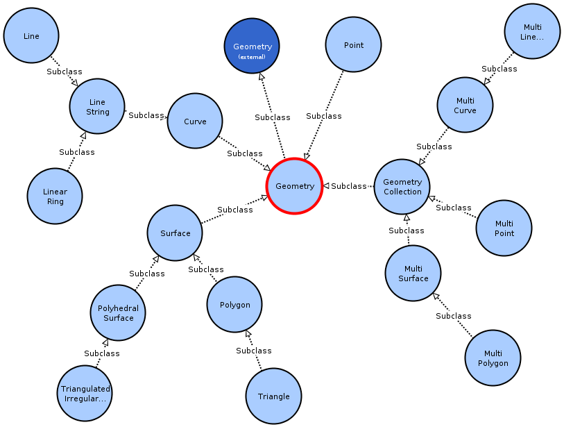
The sf:Geometry: class itself has four direct
sub-classes. Three correspond to zero, one and two -dimensional objects,
with a fourth abstracting objects composed by more than one geometric
primitive.
sf:Point: a 0-dimensional geometry instance, representing a single location in coordinate space. A point has an x-coordinate value and a y-coordinate value.sf:Curve: a 1-dimensional geometry instance, usually stored as a sequence of points. The sub-types of Curve specifies the interpolation method between points.sf:Surface: a 2-dimensional geometry instance. It may consist of a single patch that is associated with one exterior boundary and 0 or more interior boundaries.sf:GeometryCollection: a geometry instance that is a collection of some number of geometry instances.
Only one interpolation method is specified for the
sf:Curve class, with the sf:LineString
sub-class. The latter is further specified with
sf:Line:
sf:LineString: a curve with linear interpolation between points. Each consecutive pair of points defines a line segment.sf:Line: asf:LineString: instance composed of exactly twosf:Point: instances.sf:LinearRing: asf:LineString: instance that is both closed and simple.
The sf:Surface: class is specialised into
sf:PolyhedralSurface: and sf:Polygon, with
each of those further specialised into sf:TIN: and
sf:Triangle.
sf:Polygon: A planar surface defined by 1 exterior boundary and 0 or more interior boundaries.sf:Triangle: Asf:Polygon: instance with 3 distinct, non-collinear vertices and no interior boundary.sf:PolyhedralSurface: a contiguous collection of polygons, which share common boundary segments.sf:TIN: A Triangulated Irregular Network (TIN) is asf:PolyhedralSurfaceinstance composed only of triangles.
sf:GeometryCollection: is specialised into three
sub-classes identifying collections of zero, one and two dimensional
geometries. The sf:Curve: and sf:Surface:
collections are further specialised.
sf:MultiPoint: a 0-dimensionalsf:GeometryCollection: instance, i.e., all its elements aresf:Point: instances.sf:MultiCurve: a 1-dimensionalsf:GeometryCollection: instance, i.e., all its elements aresf:Curve: instances.sf:MultiLineString: Asf:MultiCurve: instance whose elements aresf:LineStringsf: instances.sf:MultiSurface: a 2-dimensionalsf:GeometryCollection: instance, i.e., all its elements aresf:Surface: instances.sf:MultiPolygon: Asf:MultiSurface: instance whose elements aresf:Polygonsf: instances.
Both WKT and GML, the initial geometry serialisations adopted in GeoSPARQL 1.0, fully support the geometry types in Simple Features. However, the other introduced with GeoSPARQL 1.1 do not (KML and GeoJSON). In particular, neither is able to represent TIN geometries. These limitations should be taken into account when serialising geometries with GeoSPARQL.
6.3 GeoSPARQL as a query language
GeoSPARQL is not only the name of a geo-spatial information ontology, it is also an extension to the SPARQL language. It provides the mechanisms to query and manipulate spatial features in a triple store.
GeoSPARQL does not add further clauses to SPARQL, therefore queries
largely retain the same structure. Instead, GeoSPARQL adds a large set
of functions, that can be used in SELECT and
FILTER statements. They are defined within the document (or
namespace) http://www.opengis.net/def/function/geosparql/,
usually abbreviated in Turtle to geof:. These functions are
broadly divided in two groups: topological and non-topological. The
former inform on relations between spatial features, whereas the latter
build new literals from existing features.
In the specification of the query language a wildcard of sorts is
used: ogc:geomLiteral. It is meant as an umbrella concept
over the five literal types (Section 6.2.2). For unknown reasons, the
OGC opted for not formalising this meta-type and only defining textually
in the documentation. In certain cases ogc:geomLiteral is
also used as a stub for geometry collection classes. To avoid confusion,
read carefully the text describing each function.
6.3.1 OGC units of measure
Several non-topological query functions return numerical literals
that refer to a unit of measure. The OGC has defined a small set of URIs
corresponding to standard units of measure, all under the path
http://www.opengis.net/def/uom/OGC/1.0/ (it can be
abbreviated to geo-uom). For example, the URI
<http://www.opengis.net/def/uom/OGC/1.0/metre>
identifies the metre. The full list of these units is:
geo-uom:amperegeo-uom:candelageo-uom:degreegeo-uom:gridspacinggeo-uom:kelvingeo-uom:kilogramgeo-uom:metregeo-uom:molegeo-uom:radiangeo-uom:secondgeo-uom:unity
The OGC maintains a small vocabulary with succinct definitions of these units of measure and links to semantically equivalent classes 15. Particularly relevant are the relations to reciprocate units of measure in the QUDT ontology (Section 3.5).
6.3.2 Non-topological functions
These functions operate on spatial features and return a literal, either numerical or geometric. They provide information such as the distance between two features or the envelope of a feature. These non-topological functions are consistent with those of the same name defined in the Simple Features ISO standard [ISO 19125-1]. This section lists these functions, their arguments and return types for quick reference.
6.3.2.1 geof:distance
geof:distance (geom1: ogc:geomLiteral,
               geom2: ogc:geomLiteral,
               units: xsd:anyURI): xsd:double
Returns the shortest distance in units between any two points in the
two geometric objects as calculated in the CRS of the first argument
(geom1).
6.3.2.2 geof:buffer
geof:buffer (geom: ogc:geomLiteral,
             radius: xsd:double,
             units: xsd:anyURI): ogc:geomLiteral
Returns a geometric object representing all points whose distance
from the first argument (geom) is less than, or equal to,
the given radius, measured in the given units.
Calculations are conducted in the spatial reference system of
geom.
6.3.2.3 geof:convexHull
geof:convexHull (geom1: ogc:geomLiteral): ogc:geomLiteralReturns a geometric object representing all points in the convex hull of the argument. Calculations are conducted in the CRS of the argument.
6.3.2.4 geof:aggConvexHull
geof:aggConvexHull (geom: ogc:geomLiteral): ogc:geomLiteralCalculates the convex hull of all geometries composing the given
literal. Operates on geometry collections such as
MultiPoligon of MultiPoint.
6.3.2.5 geof:intersection
geof:intersection (geom1: ogc:geomLiteral,
                   geom2: ogc:geomLiteral): ogc:geomLiteral
Returns a geometric object representing all points in the intersection of the two arguments. Calculations are conducted in the spatial reference system of the first argument.
6.3.2.6 geof:union
geof:union (geom1: ogc:geomLiteral,
            geom2: ogc:geomLiteral): ogc:geomLiteral
Returns a geometric object representing all points in the union of the two arguments. Calculations are conducted in the CRS of the first argument.
6.3.2.7 geof:aggUnion
geof:aggUnion (geom: ogc:geomLiteral): ogc:geomLiteralCalculates the union of all geometries composing the given literal.
Operates on geometry collections such as MultiPoligon of
MultiPoint.
6.3.2.8 geof:aggBoundingCircle
geof:aggBoundingCircle (geom: ogc:geomLiteral): ogc:geomLiteralCalculates a minimum bounding circle of all geometries composing the
given literal. Operates on geometry collections such as
MultiPoligon of MultiPoint.
6.3.2.9 geof:aggCentroid
geof:aggCentroid (geom: ogc:geomLiteral): ogc:geomLiteralCalculates the aggregate centroid of all geometries composing the
given literal. Operates on geometry collections such as
MultiPoligon of MultiPoint.
6.3.2.10 geof:difference
geof:difference (geom1: ogc:geomLiteral,
                 geom2: ogc:geomLiteral): ogc:geomLiteral
Returns a geometric object representing all points in the set difference of the two arguments. Calculations are conducted in the CRS of the first argument.
6.3.2.11 geof:symDifference
geof:symDifference (geom1: ogc:geomLiteral,
                    geom2: ogc:geomLiteral): ogc:geomLiteral
Returns a geometric object representing all points in the set symmetric difference of the two arguments. Calculations are conducted in the spatial reference system of the first argument.
6.3.2.12 geof:envelope
geof:envelope (geom1: ogc:geomLiteral): ogc:geomLiteralReturns the minimum bounding box of the argument geometry.
6.3.2.13 geof:boundary
geof:boundary (geom1: ogc:geomLiteral): ogc:geomLiteralReturns the closure of the boundary of the argument geometry.
6.3.2.14 geof:getsrid
geof:getSRID (geom: ogc:geomLiteral): xsd:anyURIReturns the URI of the CRS associated with the argument geometry.
6.3.2.15 geof:transform
geof:transform (geom: ogc:geomLiteral, srsIRI: xsd:anyURI): ogc:geomLiteralTransforms a geometry literal into a different coordinate system
defined by the srsIRI parameter. Returns an error if the
transformation is not mathematically possible.
6.3.2.16 geof:geometryN
geof:geometryN (geom: ogc:geomLiteral, geomindex: xsd:integer): ogc:geomLiteralGiven a Geometry literal composed by multiple instances,
returns the individual at the given index. Applies to instances of the
sf:GeometryCollection class,
e.g. sf:MultiPoint.
6.3.2.17 geof:numGeometries
geof:numGeometries (geom: ogc:geomLiteral): xsd:integerGiven a Geometry literal composed by multiple
individuals, returns the its total number of individuals. Applies to
instances of the sf:GeometryCollection class,
e.g. sf:MultiPoint.
6.3.2.18 Coordinates minima and maxima
GeoSPARQL 1.1 introduced six new functions returning the minima and maxima values for each coordinate, easting, northing and altitude. Their working should be evident from the signature.
geof:minX (geom: ogc:geomLiteral): xsd:doublegeof:maxX (geom: ogc:geomLiteral): xsd:doublegeof:minY (geom: ogc:geomLiteral): xsd:doublegeof:maxY (geom: ogc:geomLiteral): xsd:doublegeof:minZ (geom: ogc:geomLiteral): xsd:doublegeof:maxZ (geom: ogc:geomLiteral): xsd:double6.3.3 DE-9IM
Clementini (Clementini, Felice, and Oosterom 1993) introduced a set of topological relationships between two geometries in the Cartesian space, formalising concepts found in natural speech. They express mathematically what it means, for instance, two geometries to overlap, or share a common border. Clementini later perfected his concept (Clementini, Sharma, and Egenhofer 1994), tapping on previous work by M. J. Egenhofer and Franzosa (1991). This relation set eventually became known as the Dimensionally Extended 9-Intersection Model (DE-9IM), later adopted as a standard by ISO (“Geographic information – Simple feature access – Part 1: Common architecture” 2004). The DE-I9M became an important tool in the computation geo-spatial features.
The DE-9IM model formalises nine different relationships, relating to the interior, the boundary and exterior of two geometries. These relations are usually set up in a three-by-three matrix, with three rows for a geometry a and three columns for a second geometry b. Figure 28 presents the DE-9IM relations. For their mathematical formulation please consult Clementini (Clementini, Sharma, and Egenhofer 1994) or the ISO 19125-1 standard (“Geographic information – Simple feature access – Part 1: Common architecture” 2004).

Spatial relation patterns between two geometries, e.g. overlaps, touches, etc, can be defined with boolean realisations of the DE-9IM relationships, indicating which must be verified (True), which must not be verified (False) and which are optional (empty, usually represented with an asterisk). These patterns can be mathematically expressed in the form of a 3-by-3 matrix. Take for instance the matrix in Table tbl. 11. It declares that the intersection of the two geometries interior cannot be an area, but that the interior of the first geometry must intersect the border of the second geometry along a line.
| F T * |
| * * * |
| * * * |
For convenience, a DE-9IM pattern can also be represented in the form
of a vector transposed from the original matrix. For instance the
[T*****FF*] represents the same “contains” pattern as the
matrix in table tbl. 12.
| T * * |
| * * * |
| F F * |
6.3.3.1 geof:relate
The DE-9IM patterns are thus used in GeoSPARQL to provide an holistic
approach to geometry relation queries. A single function –
relate – allows their application to two geometries.
Listing 117 presents the signature of this function: two geometries as
inputs, plus a string with the DE-9IM pattern vector, the output is a
boolean value, indicating weather the relation is valid or not.
Listing 117: The relate function applies DE-9IM patterns to two geometries
geof:relate (geom1: ogc:geomLiteral,
             geom2: ogc:geomLiteral,
             pattern-matrix: xsd:String): xsd:boolean
6.3.3.2 Simple Features
Beyond the relate function, GeoSPARQL further provides a
roll of geometry relation functions stemming from popular standards and
literature. Among those is the family of topological relations specified
in the Simple Features standard issued by ISO [ISO 19125-1]. Their names
and equivalent DE-9IM pattern is presented in Table 13. All these
functions have the same signature, with two geometries
(ogc:geomLiteral) as input and a boolean as output
(xsd:boolean).
| Function name | DE-9IM pattern | Geometry types |
|---|---|---|
| sfEquals | (TFFFTFFFT) |
all |
| sfDisjoint | (FF*FF****) |
all |
| sfIntersects | (T*********T**********T*********T****) |
all |
| sfTouches | (FT*******F**T*****F***T****) |
all except point-point |
| sfWithin | (T*F**F***) |
all |
| sfContains | (T*****FF*) |
all |
| sfOverlaps | (T*T***T**) |
area-area, point-point |
| sfOverlaps | (1*T***T**) |
line-line |
| sfCrosses | (T*T***T**) |
point-line, point-area, line-area |
| sfCrosses | (0********) |
line-line |
6.3.3.3 Egenhofer
Another important family of geometry relation function is that proposed by (M. J. Egenhofer 1989). They apply more generally to areas, lines and points. Table 14 presents succinctly the Egenhofer functions and the corresponding DE-9IM patterns.
| Relation name | DE-9IM pattern | Geometry types |
|---|---|---|
| ehEquals | (TFFFTFFFT) |
all |
| ehDisjoint | (FF*FF****) |
all |
| ehMeet | (FT*******F**T*****F***T****) |
all except point-point |
| ehOverlap | (T*T***T**) |
all |
| ehCovers | (T*TFT*FF*) |
area-area, area-line, line-line |
| ehCoveredBy | (TFF*TFT**) |
area-area, line-area, line-line |
| ehInside | (TFF*FFT**) |
all |
| ehContains | (T*TFF*FF*) |
all |
6.3.3.4 RCC8
Finally, GeoSPAQRL specifies also the functions of the RCC8 family (Randell, Cui, and Cohn 1992). Apart from the other families, the RCC8 functions only apply to areas. Table 15 relate these functions with the corresponding DE-9IM patterns.
| Relation name | DE-9IM pattern |
|---|---|
| rcc8eq | (TFFFTFFFT) |
| rcc8dc | (FFTFFTTTT) |
| rcc8ec | (FFTFTTTTT) |
| rcc8po | (TTTTTTTTT) |
| rcc8tppi | (TTTFTTFFT) |
| rcc8tpp | (TFFTTFTTT) |
| rcc8ntpp | (TFFTFFTTT) |
| rcc8ntppi | (TTTFFTFFT) |
GeoSPARQL provides a wide range of options to query a geo-spatial triple store with topology functions. Either with the DE-9IM patterns or the three function families on offer there are multiple avenues to relate two geometries.
6.3.4 Geometry conversion functions
These functions provide the mechanisms to transform one literal
geometry serialisation into another. Their workings should be evident,
e.g. asWKT transforms whichever argument geometry literal
into an instance of the WKTLiteral type.
geof:asWKT (geom: ogc:geomLiteral): geo:wktLiteralgeof:asGML (geom: ogc:geomLiteral, gmlProfile: xsd:string): geo:gmlLiteralThe transformations into GeoJSON and KML must be applied with extra care, as they may imply a datum transformation into CRS84. Make sure the input geometry justify such transformation, how the software performs it and how it reports transformation uncertainty.
geof:asGeoJSON (geom: ogc:geomLiteral): geo:geoJSONLiteralgeof:asWKT (geom: ogc:geomLiteral): geo:wktLiteralRegarding the asDGGS transformation it is anyone’s guess
its exact meaning. In case you ever come across a software package
implementing this function take extra precaution understanding its
working and the kinds of DGGSs it may support.
geof:asDGGS (geom: ogc:geomLiteral, specificDggsDatatype: xsd:anyURI): geo:DggsLiteral6.4 Geo-spatial data with GeoSPARQL
The best way to get acquainted with geo-spatial data in the Semantic Web is by conducting a small trial. From simple geometries digitised over a map, this section takes you through the steps necessary to arrive at geo-spatial RDF. In first place it is necessary to create an ontology providing the semantics to data individuals. Then you will see how to use GeoSPARQL to add the geo-spatial dimension to those individuals.
The ontology in the example below (Listing 118) is an extension to the ontology developed in Chapter 3 and is henceforth referred as Mobility Geography. It introduces spatial features related to recreational cycling, going through points, lines and polygons. They are:
Nature areas: polygons marking areas wherein wildlife is protected, and in which humans recreate themselves hiking, running, cycling, etc.
Cycle paths: lines marking paths, usually paved, made for cycling and safe from motorised traffic.
Landmarks: sites in the landscape worth visiting, either for sight seeing or giving access to a particular monument.
Listing 118: Geo-spatial classes in the Mobility ontology
@prefix : <https://www.linked-sdi.com/mobility-geo#> .
@prefix xsd: <http://www.w3.org/2001/XMLSchema#> .
@prefix rdf: <http://www.w3.org/1999/02/22-rdf-syntax-ns#> .
@prefix rdfs: <http://www.w3.org/2000/01/rdf-schema#> .
@prefix owl: <http://www.w3.org/2002/07/owl#> .
@prefix geo: <http://www.opengis.net/ont/geosparql#> .

<https://www.linked-sdi.com/mobility-geo> rdf:type owl:Ontology .

:Landmark rdf:type owl:Class ;
          rdfs:subClassOf geo:Feature ;
          rdfs:label "Landmark"@en ;
          rdfs:comment
               """ A remarkable location in the landscape,
                   offering an exceptional view, signalling a
                   natural or human monument, or simply a place
                   to rest. """@en .

:CyclePath rdf:type owl:Class ;
           rdfs:subClassOf geo:Feature ;
           rdfs:label "Cycle Path"@en ;
           rdfs:comment
                """ A paved path for the exclusive use by pedal
                    and human powered vehicles. In some countries
                    low powered motorcycles may be allowed too.
                """@en .

:NatureArea rdf:type owl:Class ;
            rdfs:subClassOf geo:Feature ;
            rdfs:label "Nature Area"@en ;
            rdfs:comment
                 """ A delimited area where most human activities
                     are forbidden (e.g. camping, farming,
                     hunting, fishing, etc) and fauna and flora
                     are left to develop with little to no
                     management."""@en .
The following step is to add a few properties to these classes. For
the Landmark class the property facilities
indicates whether some resupply amenities exist, somewhere to have a
comfort break or get a snack from. For the CyclePath class
it is important to know if access is paid or free of charge, hence the
freeAccess property. The properties in Listing 119
exemplify how the counterpart of an attribute table is built in the
Semantic Web.
Listing 119: Properties for geo-spatial classes in the Mobility ontology
:facilities rdf:type owl:DatatypeProperty ;
            rdfs:domain :Landmark ;
            rdfs:range xsd:boolean ;
            rdfs:label "Facilities"@en ;
            rdfs:comment
                 """ Indicates whether in the viccinity of a
                     landmark infrastructure(s) exist(s),
                     allowing for a confort break, a snack or
                     bicycle repairs. """@en .

:freeAccess rdf:type owl:DatatypeProperty ;
            rdfs:domain :NatureArea ;
            rdfs:range xsd:boolean ;
            rdfs:label "Free access"@en ;
            rdfs:comment
                 """ Indicates whether a nature area is freely
                     accessible or not."""@en .
For the CyclePath class it is relevant to know the kind
of surface (it could influence your choice of bicycle). The
pavemenType object property creates a relationship with the
Pavement enumerate, as Listing 120 shows. The complete
Mobility Geography ontology can be consulted in Annex C.
Listing 120: Enumetare for geo-spatial classes in the Mobility ontology
:Pavement rdf:type owl:Class ;
          owl:oneOf (:tarmac :concrete :gravel) ;
          rdfs:label "Pavement"@en ;
          rdfs:comment "Type of pavement in cycle paths"@en .

:tarmac rdf:type :Pavement ;
        rdfs:label "Tarmac"@en ;
        rdfs:comment
             """ Fast but grippy surface composed of a misture of
                 concrete and bitumen. """@en .

:concrete rdf:type :Pavement ;
          rdfs:label "Concrete"@en ;
          rdfs:comment
               """ A pavement composed of concrete blocks. Fast
                   and smooth surface. Usually less grippier in
                   the wet, unless groved. """@en .

:gravel rdf:type :Pavement ;
        rdfs:label "Gravel"@en ;
        rdfs:comment
             """ A dirt surface covered with some degree of
                 gravel stones. Slippery and prone to sogginess
                 in the rain. """@en .

:pavementType rdf:type owl:ObjectProperty ;
              rdfs:domain mob:CyclePath ;
              rdfs:range mob:Pavement .
6.4.1 Obtain WKT from a OGR supported file format
Equipped with a new ontology for recreational cycling, you can now
move on to encode actual geo-spatial data. The spatial features in this
example are sited in the Gelderland region. The resulting knowledge
graph assumes the same name, with the URI
<https://www.linked-sdi.com/gelderland>. The complete
Gelderland knowledge graph can be consulted in Annex D.
With the ontology defined it is now time to start creating some
actual features composing a knowledge graph. Doing so requires the WKT
of the corresponding geometries, which most possibly are stored in a
household vector file format like GeoPackage. There are various ways of
doing so, but perhaps the simplest is to issue SQL queries directly to
the source file with OGR. Listing 121 shows how to obtain the feature id
and the corresponding geometry from a GeoPackage file16
using the SQL facilities provided by SpatiaLite. If instead you still
use the outdated Shapefile format, you may use the special field
OGR_GEOM_WKT to obtain the WKT for a geometry.
Listing 121: Obtain the WKT for a geometry using the ogrinfo tool
$ ogrinfo "Landmarks.gpkg" -geom=yes -sql "SELECT *, AsWKT(CastAutomagic(geom)) FROM Landmarks"
INFO: Open of `Landmarks.gpkg'
      using driver `GPKG' successful.

Layer name: SELECT
Geometry: None
Feature Count: 6
Layer SRS WKT:
(unknown)
FID Column = fid
geom: String (0.0)
id: Integer64 (0.0)
name: String (80.0)
AsWKT(CastAutomagic(geom)): String (0.0)
OGRFeature(SELECT):1
  geom (String) = GP
  id (Integer64) = (null)
  name (String) = Radio Kotwijk
  AsWKT(CastAutomagic(geom)) (String) = POINT(5.81964098736039 52.17349648003406)

OGRFeature(SELECT):2
  geom (String) = GP
  id (Integer64) = (null)
  name (String) = Posbank
  AsWKT(CastAutomagic(geom)) (String) = POINT(6.021252376222333 52.02848711149809)

OGRFeature(SELECT):3
  geom (String) = GP
  id (Integer64) = (null)
  name (String) = Zijpenberg
  AsWKT(CastAutomagic(geom)) (String) = POINT(6.005032119303396 52.02589802195161)

OGRFeature(SELECT):4
  geom (String) = GP
  id (Integer64) = (null)
  name (String) = Lentse Warande
  AsWKT(CastAutomagic(geom)) (String) = POINT(5.867091831858774 51.85683804524761)

OGRFeature(SELECT):5
  geom (String) = GP
  id (Integer64) = (null)
  name (String) = Berg en Dal
  AsWKT(CastAutomagic(geom)) (String) = POINT(5.915006360672288 51.82480437041511)

OGRFeature(SELECT):6
  geom (String) = GP
  id (Integer64) = (null)
  name (String) = Mossel
  AsWKT(CastAutomagic(geom)) (String) = POINT(5.7614399118364 52.0622661566825)
6.4.2 Create a Landmark feature with associated point geometry
Having obtained the WKT for the geometry, it is now possible to create the corresponding feature instance and associated geometry (Listing 122).
Listing 122: Landmark feature and corresponding geometry
@prefix rdfs:  <http://www.w3.org/2000/01/rdf-schema#> .
@prefix geo: <http://www.opengis.net/ont/geosparql#> .
@prefix mob-geo: <https://www.linked-sdi.com/mobility-geo#> .
@prefix gelre: <https://www.linked-sdi.com/gelderland#> .

gelre:radioKotwijkGeom a geo:Geometry, sf:Point ;
    geo:asWKT "POINT(5.7614399118364 52.0622661566825)"^^geo:wktLiteral .

gelre:radioKotwijk a mob-geo:Landmark ;
    rdf:label "Radio Kotwijk"@en ;
    geo:hasGeometry gelre:radioKotwijkGeom ;
    mob-geo:facilities "false"^^xsd:boolean ;
For the cycle paths the same pattern applies, first declaring the Geometry instance and encoding it and then creating the corresponding Feature. Listing 123 shows an example with an instance of the CyclePath class.
Listing 123: CyclePath feature and corresponding geometry
@prefix rdfs:  <http://www.w3.org/2000/01/rdf-schema#> .
@prefix geo: <http://www.opengis.net/ont/geosparql#> .
@prefix mob-geo: <https://www.linked-sdi.com/mobility-geo#> .
@prefix gelre: <https://www.linked-sdi.com/gelderland#> .

gelre:zevendalsewegkGeom a geo:Geometry, sf:Line ;
    geo:asWKT "LINESTRING(5.919891267657165 51.73823051725662,5.919863174950073 51.73831749995509,5.918805016316298 51.73837548832774,5.917859228510888 51.73832329879571,5.91733483131185 51.73852625774832,5.917306738604758 51.7391525253414,5.915658633122064 51.74002812566536,5.910901601387925 51.74183725934144,5.90929095284802 51.74288095735793,5.908298343864125 51.74303171174529,5.90743683417999 51.74373909099881,5.908935111891529 51.74612786367065,5.909496966033356 51.74684099219383,5.910639402788405 51.7507485047321,5.910639402788405 51.75175721420073,5.910264833360521 51.75291662254316,5.909796621575664 51.75457452476162,5.909553151447539 51.75510782302704,5.908795818885969 51.75570089257475,5.908065408501674 51.75580523143283,5.907475461652821 51.75615302588536,5.905354462267655 51.75793543041366,5.901477668689473 51.76128268293113)"^^geo:wktLiteral .

gelre:zevendalseweg a mob-geo:CyclePath ;
    rdf:label "Zevendalseweg"@en ;
    geo:hasGeometry gelre:zevendalsewegGeom ;
    mob-geo:pavement mob-geo:tarmac .
At this point things are becoming fairly verbose, thanks to the nature of WKT and the excessive precision of the coordinates stored in the original format. It is easy to see how this task of creating GeoSPARQL can rapidly become tedious. Some sort of automation is thus in order, which is the topic tackled in Chapter 7.
6.4.3 Querying a Geo-spatial Knowledge Graph
With a complete knowledge graph in the triple store, it is now
possible to create geo-spatial queries. Listing 124 finds the answer to
the question: “which landmarks are within a nature area”? The
formulation is not complex, first match individuals for
Landmark and CyclePath, then match their
respective geometries. With the latter, the geometry literals are
matched and finally used within a FILTER clause with the
sfIntersects function. The output of this query is shown in
Listing 125. Note that building this kind of query requires prior
knowledge on the kind of serialisation used for the geometry literals.
If these geometries were serialised as GML literals, the triples in
Listing 124 with the geo:asWKT predicate would not match
any literals and the query would return an empty result.
Listing 124: Identifying landmarks within nature areas
PREFIX geo: <http://www.opengis.net/ont/geosparql#>
PREFIX mob-geo: <https://www.linked-sdi.com/mobility-geo#>

SELECT ?l ?a
WHERE {
    ?l a mob-geo:Landmark ;
        geo:hasGeometry ?geom_l .
    ?a a mob-geo:CyclePath ;
        geo:hasGeometry ?geom_a .
    ?geom_l geo:asWKT ?wkt_l .
    ?geom_a geo:asWKT ?wkt_a .
    FILTER(geo:sfIntersects(?wkt_l, ?wkt_a))
}
Listing 125: Result to query in [Listing @lst:geo:ex:landmarksNature]
LONG VARCHAR                                           LONG VARCHAR
___________________________________________________________________

https://www.linked-sdi.com/gelderland#posbank          https://www.linked-sdi.com/gelderland#veluwezoom
https://www.linked-sdi.com/gelderland#zijpenberg       https://www.linked-sdi.com/gelderland#veluwezoom
Another example, answering the question: “which landmarks lay close
to interesting cycle paths”? In this case there is an intersection to
test between Point and Line geometries, which
is likely to return empty. An approach to this case is to use a buffer,
for instance around the Landmark literals. But since these
literals are defined on a geographic SRS a caveat must be considered: if
the buffer is defined in degrees, it wont produce a symmetrical circle
around the point. This is where the units argument to the
geof:buffer functions helps, in Listing 126 a distance of
500 metres is applied.
Listing 126: Identifying landmarks close to cycle paths
PREFIX geo: <http://www.opengis.net/ont/geosparql#>
PREFIX geof: <http://www.opengis.net/def/function/geosparql/>
PREFIX mob-geo: <https://www.linked-sdi.com/mobility-geo#>
SELECT ?l ?p
WHERE {
    ?l a mob-geo:Landmark ;
        geo:hasGeometry ?geom_l .
    ?p a mob-geo:CyclePath ;
        geo:hasGeometry ?geom_p .
    ?geom_l geo:asWKT ?wkt_l .
    ?geom_p geo:asWKT ?wkt_p .
    FILTER(geof:distance(?wkt_l, ?wkt_p, <http://www.opengis.net/def/uom/OGC/1.0/metre>) < 500)
}
As is usual in geo-spatial analysis, there is more than one way to reach the same answer. Listing 127 provides a different formulation to identify landmarks in reach of cycle paths.
Listing 127: Identifying landmarks close to cycle paths in a different way
PREFIX geo: <http://www.opengis.net/ont/geosparql#>
PREFIX geof: <http://www.opengis.net/def/function/geosparql/>
PREFIX mob-geo: <https://www.linked-sdi.com/mobility-geo#>
SELECT ?l ?p
WHERE {
    ?l a mob-geo:Landmark ;
        geo:hasGeometry ?geom_l .
    ?p a mob-geo:CyclePath ;
        geo:hasGeometry ?geom_p .
    ?geom_l geo:asWKT ?wkt_l .
    ?geom_p geo:asWKT ?wkt_p .
    FILTER(geof:buffer(?wkt_l, ?wkt_p, <http://www.opengis.net/def/uom/OGC/1.0/metre>) < 500)
}
6.5 Coordinate References Systems
6.5.1 General
As the old adage goes, spatial data without a reference system or reference frame is only spatial in name. Section 6.2 briefly introduced the mechanism used in GeoSPARQL to express the CRS encoding, concatenating a CRS URI with the WKT or GML encoding of the geometry itself. In fact that is all there is to it, the standard does not provide guidance on the structure of that URI, much less on the kind of information it may provide in case it is derreferenceable. CRSs are definitely work in progress in the Semantic Web, and whereas it is possible to publish geo-spatial linked data in an accurate and unequivocal manner, there are plenty of pitfalls along the way.
Geo-spatial standards for the web such GeoSPARQL, GML or GeoJSON have historically favoured geodesic (or geographic) coordinate systems. I.e. positioning on the surface of a solid approximating the Earth’s surface (the datum), indexed with a latitude-longitude coordinate pair. This is in contrast to projected (or cartographic) coordinate systems, where spatial positioning is established with a easting-northing pair referring to a flat surface. This makes perfect sense in an age where receivers of satellite positioning systems have become so ubiquitous (you probably own more than one). However, this trend has created two important issues for geo-spatial data on the web: the ambiguity of datum definitions and the misinterpretation of axes order in geodesic coordinate systems. Before getting into the specifics of GeoSPARQL it is important to revisit those.
6.5.2 The WGS84 datum series
If you ever worked with data acquired with a GPS receiver you probably have come across the WGS84 CRS, usually identified with the code 4326 in the index of the European Petroleum Survey Group (EPSG) 17. But what exactly does it represent?
At the beginning of the 1980s computers were becoming ubiquitous in the corporate world, paving the way for the new geo-spatial applications based on digital infrastructures. At the same time, launching satellites into Earth’s orbit was becoming common place, with the Global Positioning System (GPS) coming on-line, and on the verge of being open to the public. The onset of this new digital age prompted the definition of global geodetic system with considerably more parameters and detail than before. Responsible for the GPS project, the United States Department of Defence naturally lead the way, with the National Geospatial-Intelligence Agency (NGA) establishing the World Geodetic System in 1984. It includes a detailed ellipsoid and various gravimetric parameters, forming a datum centered on the Earth’s centre of mass. The NGS has maintained the WGS84 since 1984.
The keyword in the little story above is “maintained”. The WGS84 is an attempt at a one-size-fits-all datum to be used around world. But the Earth is a pretty lively beast, with plate tectonics constantly modifying its outer shape. Take the Atlantic rift for instance, Europe and North America move apart 2.5 cm every year. Other tectonic plates move even faster. Every few years the datum needs to be slightly repositioned, so that it meets again its original criteria. Each update creates a new WGS84 reference frame, religiously documented by the NGA. For this reason the WGS84 is referred as a dynamic datum, a datum series or a datum ensemble. Table 16 lists the reference frames published so far and their individual codes in the EPSG index.
In effect, when you refer the WGS84 without specifying a particular reference frame, for instance by stating solely the EPSG code 4326, you are in practice referring to seven different datums. This translates into a visible positional uncertainty. The same pair of coordinates can refer to positions various metres apart, whether it is realised by the early 1984 reference frame or the latest published in 2021. While for many applications this may be an acceptable uncertainty, it can easily be a problem in legally bound contexts, for example, determining the location of a natural resource on a cadastre.
Whenever you use the WGS84 ensemble (EPSG:4326) with your digital data, you are offloading on the software the responsibility to select one of the datums in the series. This may lead to unexpected results if the datum selected by the software does not match the one used to acquire the original positioning. And with the publication of further updates to the series by the NGA this problem only becomes worse with time.
Although still ubiquitous, awareness of this sloppy use of the WGS84 is slowly emerging. The also ubiquitous GDAL/OGR geo-spatial data abstraction library today sports a caution note against the use of the WGS84 series in its manual (Warmerdam, Rouault, and alia 2022), recommending the direct reference to one of the specific reference frames instead. European institutions also discourage the use of the WGS84 series, legally binding directives such as INSPIRE recommend the ETRS89 datum.
| EPSG code | WGS84 Reference frame | Year |
|---|---|---|
| 8888 | Transit | 1984 |
| 9053 | G730 | 1994 |
| 9054 | G873 | 1997 |
| 9055 | G1150 | 2002 |
| 9056 | G1674 | 2012 |
| 9057 | G1762 | 2015 |
| 9755 | G2139 | 2021 |
6.5.3 The order of coordinates in geodesic CRSs
Determining the latitude of a place is a simple exercise that geographers and navigators have practised for millennia (most notably Erathosthenes in the experiment that lead to the first accurate estimate of the size of the Earth). Either by measuring the angle of the Sun, the Northern Star or the Southern Cross with the horizon a precise measurement can be obtained. However, estimating longitude with precision remained an elusive exercise up to the late XVIII century, when John Harrison produced the first maritime chronograph. For this reason cartographers have reported geodesic coordinates in the latitude-longitude order, first the most and then the least accurate.
And so it went until computers came into the picture. Perhaps failing to grasp the fundamental differences between cartographic and geodesic coordinate systems, early geo-spatial software makers misinterpreted geodetic coordinate pairs and chaos soon set in. Geodesic coordinates report angles of normal vectors with the surface of the planet, they do not refer to Cartesian axes, but still this problem became known as the “axis [sic] order confusion”. Whereas cartographers and geodesists report as latitude-longitude pairs, software interprets them as longitude-latitude.
Early on the OGC made coordinate order explicit in its specifications, declaring the first (or “X”) coordinate to represent latitude and not longitude with geodesic CRSs. But few software packages complied with these specifications. When it released version 1.3 of the WMS standard the OGC specified a new CRS attempting to deal with this problem, adopting the WGS84 datum but with an inverted coordinate order, longitude first, latitude second (La Beaujardiere 2006). This CRS has been known as “CRS:84”, “OGC:CRS84”, but today is mostly referred simply as “CRS84”. CRS84 was adopted as default CRS in the GeoJSON specification (and eventually as only allowed CRS) and also in GeoSPARQL. Debate is still alive on whether CRS84 helped solved the issue, or actually made it worse. It does not help the OGC not being clear if CRS84 refers to the full WGS84 datum ensemble or only to its first reference frame.
Eventually, the EPSG felt compelled to explicitly record axes order in its CRS registry. Hopefully this would force software makers to comply. Both the OGC and ISO would acknowledge this need, adopting the philosophy of the EPSG. The specification of the Well Known Text (WKT) format for CRS encoding well accommodates this requirement (in a similar way to the earlier textual specification from the OGC). The OGC went as far as releasing a policy statement declaring the need for digital coordinate systems to explicitly declare coordinates order (Board 2017). The Simple Features, GeoSPARQL and GML specifications are all clear in this regard: geometries are encoded with the coordinates order declared by the CRS.
However, the confusion prevails to this day, with many software packages still misinterpreting the order of geodesic coordinates, implicitly assuming they refer to Cartesian axes.
6.5.4 Example
To illustrate the lingering difficulties in working with geodetic CRSs this section provides a simple example with a GPX file. In Listing 128 is a minimalistic file with a single point geometry that could be obtained from any GPS receiver.
Listing 128: Contents of a simple GPX with a single way point.
<gpx version="1.0">
  <wpt lat="45" lon="-120"></wpt>
</gpx>
The first exercise is to transform this file into the GML format,
which could be used as literal in a GeoSPARQL knowledge graph. Listing
129 shows how to do so with the useful ogr2ogr
transformation utility from the GDAL/OGR software package. Note the
correct identification of a the CRS with a URN (more on that latter in
this section) and the coordinates correctly encoded with latitude first
and longitude second.
Listing 129: Successful transformation of a sample GPX file to GML with OGR.
$ ogr2ogr -f GML waypoint.gml waypoint.gpx

$ cat waypoint.gml
<?xml version="1.0" encoding="utf-8" ?>
<ogr:FeatureCollection
     gml:id="aFeatureCollection"
     xmlns:xsi="http://www.w3.org/2001/XMLSchema-instance"
     xsi:schemaLocation="http://ogr.maptools.org/ waypoint.xsd"
     xmlns:ogr="http://ogr.maptools.org/"
     xmlns:gml="http://www.opengis.net/gml/3.2">
  <gml:boundedBy><gml:Envelope srsName="urn:ogc:def:crs:EPSG::4326"><gml:lowerCorner>45 -120</gml:lowerCorner><gml:upperCorner>45 -120</gml:upperCorner></gml:Envelope></gml:boundedBy>

  <ogr:featureMember>
    <ogr:waypoints gml:id="waypoints.0">
      <gml:boundedBy><gml:Envelope srsName="urn:ogc:def:crs:EPSG::4326"><gml:lowerCorner>45 -120</gml:lowerCorner><gml:upperCorner>45 -120</gml:upperCorner></gml:Envelope></gml:boundedBy>
      <ogr:geometryProperty><gml:Point srsName="urn:ogc:def:crs:EPSG::4326" gml:id="waypoints.geom.0"><gml:pos>45 -120</gml:pos></gml:Point></ogr:geometryProperty>
    </ogr:waypoints>
  </ogr:featureMember>
</ogr:FeatureCollection>
Now instead of transforming into GML the next exercise creates a
GeoPackage file, also with the ogr2ogr utility. Listing 130
shows the result of consulting the resulting GeoPackage file directly
with SpatiaLite. The function AsGML returns the GML
encoding of the point geometry with swapped coordinates, longitude first
and latitude second. This is contrary to the order defined by the CRS
itself, in what is effectively an invalid geometry. In general,
SpatiaLite (and GeoPackage) should not be used with traditional geodetic
coordinate systems. CRSs with explicitly inverted coordinate order are
safe though, such as the CRS84.
Listing 130: Transformation of a sample GPX file to Geopackage mis-interpretes coordinatees order.
$ ogr2ogr -f GPKG waypoint.gpkg waypoint.gpx
$ sqlite3 waypoint.gpkg
SQLite version 3.37.2 2022-01-06 13:25:41
Enter ".help" for usage hints.

sqlite> SELECT load_extension("mod_spatialite");

sqlite> select AsGML(CastAutomagic(geom)) from waypoints;
<gml:Point srsName="EPSG:4326"><gml:coordinates>-120,45</gml:coordinates></gml:Point>
Listing 131 provides a similar example, this time with PostGis. The
waypoint GPX file is imported by ogr2ogr without issue. The
programme creates a detailed table all by itself, with dozens of
attributes. Contrary to SpatiaLite (and GeoPackage), Postgis appears to
record internally these coordinates in the correct order. However,
things are not as smooth reporting or transforming these geometries.
PostGis provides the function ST_AsGML to transformation to
GML. When used by default ST_AsGML returns invalid
geometries with swapped coordinates (line 9 in Listing 131). But using
the additional options parameter to ST_AsGML it is possible
to obtain the correct GML output (lines 11 to 14). The same does not
apply to ST_EWKT, that always transforms geometries to the
WKT format with the swapped coordinate order.
Listing 131: Transformation of a sample GPX file to PostGis and how to obtain coordinates in the correct order.
$ ogr2ogr -f "PostgreSQL" PG:"dbname=my_db" "waypoint.gpx" -nln waypoint
$ pdql -d my_db
psql (14.4 (Ubuntu 14.4-1.pgdg22.04+1))
Type "help" for help.

my_db=# select ST_AsGML(3, wkb_geometry, 2) from waypoint;
                                        st_asgml
----------------------------------------------------------------------------------------
 <gml:Point srsName="EPSG:4326"><gml:pos srsDimension="2">-120 45</gml:pos></gml:Point>
(1 row)

my_db=# select ST_AsGML(3, wkb_geometry, 2, 17) from waypoint;
                                                st_asgml
---------------------------------------------------------------------------------------------------------
 <gml:Point srsName="urn:ogc:def:crs:EPSG::4326"><gml:pos srsDimension="2">45 -120</gml:pos></gml:Point>
(1 row)

my_db=# select ST_AsEWKT(wkb_geometry) from waypoint;
        st_asewkt
--------------------------
 SRID=4326;POINT(-120 45)
(1 row)
Section 7.2 provides further cues on the transformation of geometries from traditional GIS sources such as PostGis or GeoPackage into GeoSPARQL. The goal in this sub-section is to point the perils of working with a geodetic CRS on this kind of software.
6.5.5 Registries
GeoSPARQL specifies CRS84 as the default CRS in case no URI is
provided together with the geometry WKT/GML literal. As seen in Section
6.2, an empty CRS URI equates to the
<http://www.opengis.net/def/crs/OGC/1.3/CRS84> URL.
But what if you need to encode geometries expressed with in a different
CRS (a likely necessity)? That is where CRS registries come to help.
The OGC maintains a registry of CRS URIs at
http://www.opengis.net/def/crs. Within that space, EPSG CRS
definitions can be referenced with an URI like
<http://www.opengis.net/def/crs/EPSG/0/4258>. The OGC
also serves its own CRSs (like
<http://www.opengis.net/def/crs/OGC/1.3/CRS84>) which
can not be dereferenced.
6.5.6 OGC CRS URNs
Among its many missions, the OGC maintains a registrar of names, providing unambiguous and controlled access to the consortium’s documents, namespaces and ontologies. This work is conducted by the OGC Naming Authority (OGC-NA). In its Name Type Specification (Simon Cox 2019) the OGC defines specific structures for CRS URNs and URIs that perfectly align with the GeoSPARQL specification (beyond many other benefits).
The broad idea is to provide Semantic Web friendly identifiers for
controlled CRS registries, in particular that of the EPSG. Each URI
identifies an authority, the institution responsible for the
registry, a version number and finally the code of the
CRS within the registry. An additional element, objectType
allows the OGC to distinguish URIs of different types of resources. In
this manuscript only those relative to CRSs are considered, in which the
objectType always takes the value crs. Listings
132 and Listing 133 provide the archetypes of these URIs and URNs.
Listing 132: Archetype URI for a OGC name.
http://www.opengis.net/def/objectType/authority/version/code Listing 133: Archetype URN for a OGC name.
urn:ogc:def:objectType:authority:version:code In this chapter you have already made acquaintance with the most
common of the OGC CRS URIs:
http://www.opengis.net/def/crs/OGC/1.3/CRS84. The
OGC segment identifies the authority, 1.3 the
version (a reference to version 1.3 of the WMS specification) and
CRS84 is the code. The URN formulation for this same CRS is
then urn:ogc:def:crs:OGC:1.3:CRS84. Note the capitals used
in the authority component.
To reference a CRS from the EPSG registry a similar formulation is
used, with EPSG in the authority component. Since
the EPSG definitions are not verioned, the character 0 is
used in the version component. The URI
http://www.opengis.net/def/crs/EPSG/0/3035 identifies the
EPSG:3035 CRS. The same CRS can be referred with the
urn:ogc:def:crs:EPSG:3035 (the version component
can be empty in the URN formulation.
The OGC URIs with the OGC and EPSG authorities are derefereceable. An OGC service returns a document with the GML definition of the CRS, making it rather useful as resources in RDF documents and knowledge graphs.
The OGC maintains a controlled list of authorities reachable through
the URI http://www.opengis.net/register/ogc-na/authority
(although at the time of this writting the service is down). As for the
CRS codes themselves, currently no mechanism seems to be in place to
query the OGC CRS registry.
6.5.7 Creating a CRS definition
The EPSG registry has become an ubiquitous feature of GIS, with most software able to recognise its codes to some extent. However, this registry is not by any means extensive. In comparison, the ESRI CRS registry is several times larger (ESRI 2022). In general, CRSs meant for global mapping and/or composed by cartographic projections published this side of 1900 do not feature in the EPSG registry. The EPSG is primarily focused on regional/national CRSs and classical map projections, possibly those most relevant to the Petroleum and Gas industry.
If you work with global environmental data, for instance, and wish to apply a modern and efficient equal-area projection such as those developed by Max Eckert, there is no entry in the EPSG registry to help you. In similar cases you will need to publish yourself the CRSs as a resource. That is not a difficult task, just a matter of deploying a text file to a web server. The question is rather which content should the file include.
As it happens the GeoSPARQL ontology is not normative in this sense, a URI is necessary to a CRS definition, but its exact content is left open to interpretation. The OGC is currently working on filling in this gap, and at some point it might issue an addendum to GeoSPARQL, or a new RDF-based CRS ontology altogether18.
The sensible thing to do is then to publish a CRS definition that
software can easily deal with. WKT and GML are obvious choices. The Proj
library includes a utility named projinfo that generates
such definition in WKT and JSON, the latter in various of the associated
versions. Listing 134 shows an example with one of the CRSs in the ESRI
registry, the -o parameter specifies the desired output
format, whereas the -k crs parameter requests the full
definition.
projinfo does not provide the option to generate GML.
While not necessarily an issue, you might still wish to obtain a CRS
definition in the same format as that used by the OGC in its CRS
registry. Opportunely, the GDAL library includes a similar utility,
named gdalsrsinfo, providing exactly that functionality.
Listing 135 furnished an example with the same CRS. The GML output is
far more verbose than WKT, but it is a native web format.
Listing 134: Generating a CRS definition in WKT format using `projinfo`.
$ projinfo ESRI:54052 -o wkt2:2015 -k crs
WKT2:2015 string:
PROJCRS["World_Goode_Homolosine_Land",
    BASEGEODCRS["WGS84",
        DATUM["World Geodetic System 1984",
            ELLIPSOID["WGS84",6378137,298.257223563,
                LENGTHUNIT["metre",1]]],
        PRIMEM["Greenwich",0,
            ANGLEUNIT["Degree",0.0174532925199433]]],
    CONVERSION["World_Goode_Homolosine_Land",
        METHOD["Goode Homolosine"],
        PARAMETER["Longitude of natural origin",0,
            ANGLEUNIT["Degree",0.0174532925199433],
            ID["EPSG",8802]],
        PARAMETER["False easting",0,
            LENGTHUNIT["metre",1],
            ID["EPSG",8806]],
        PARAMETER["False northing",0,
            LENGTHUNIT["metre",1],
            ID["EPSG",8807]]],
    CS[Cartesian,2],
        AXIS["(E)",east,
            ORDER[1],
            LENGTHUNIT["metre",1]],
        AXIS["(N)",north,
            ORDER[2],
            LENGTHUNIT["metre",1]],
    AREA["World"],
    BBOX[-90,-180,90,180],
    ID["ESRI",54052]]
Listing 135: Generating a CRS definition in GML format using `gdalsrsinfo`.
$ gdalsrsinfo ESRI:54052 -o xml

<gml:ProjectedCRS gml:id="ogrcrs1">
  <gml:srsName>World_Goode_Homolosine_Land</gml:srsName>
  <gml:srsID>
    <gml:name codeSpace="urn:ogc:def:crs:ESRI::">54052</gml:name>
  </gml:srsID>
  <gml:baseCRS>
    <gml:GeographicCRS gml:id="ogrcrs2">
      <gml:srsName>WGS84</gml:srsName>
      <gml:usesEllipsoidalCS>
        <gml:EllipsoidalCS gml:id="ogrcrs3">
          <gml:csName>ellipsoidal</gml:csName>
          <gml:csID>
            <gml:name codeSpace="urn:ogc:def:cs:EPSG::">6402</gml:name>
          </gml:csID>
          <gml:usesAxis>
            <gml:CoordinateSystemAxis gml:id="ogrcrs4" gml:uom="urn:ogc:def:uom:EPSG::9102">
              <gml:name>Geodetic latitude</gml:name>
              <gml:axisID>
                <gml:name codeSpace="urn:ogc:def:axis:EPSG::">9901</gml:name>
              </gml:axisID>
              <gml:axisAbbrev>Lat</gml:axisAbbrev>
              <gml:axisDirection>north</gml:axisDirection>
            </gml:CoordinateSystemAxis>
          </gml:usesAxis>
          <gml:usesAxis>
            <gml:CoordinateSystemAxis gml:id="ogrcrs5" gml:uom="urn:ogc:def:uom:EPSG::9102">
              <gml:name>Geodetic longitude</gml:name>
              <gml:axisID>
                <gml:name codeSpace="urn:ogc:def:axis:EPSG::">9902</gml:name>
              </gml:axisID>
              <gml:axisAbbrev>Lon</gml:axisAbbrev>
              <gml:axisDirection>east</gml:axisDirection>
            </gml:CoordinateSystemAxis>
          </gml:usesAxis>
        </gml:EllipsoidalCS>
      </gml:usesEllipsoidalCS>
      <gml:usesGeodeticDatum>
        <gml:GeodeticDatum gml:id="ogrcrs6">
          <gml:datumName>WGS_1984</gml:datumName>
          <gml:datumID>
            <gml:name codeSpace="urn:ogc:def:datum:EPSG::">6326</gml:name>
          </gml:datumID>
          <gml:usesPrimeMeridian>
            <gml:PrimeMeridian gml:id="ogrcrs7">
              <gml:meridianName>Greenwich</gml:meridianName>
              <gml:greenwichLongitude>
                <gml:angle uom="urn:ogc:def:uom:EPSG::9102">0</gml:angle>
              </gml:greenwichLongitude>
            </gml:PrimeMeridian>
          </gml:usesPrimeMeridian>
          <gml:usesEllipsoid>
            <gml:Ellipsoid gml:id="ogrcrs8">
              <gml:ellipsoidName>WGS84</gml:ellipsoidName>
              <gml:ellipsoidID>
                <gml:name codeSpace="urn:ogc:def:ellipsoid:EPSG::">7030</gml:name>
              </gml:ellipsoidID>
              <gml:semiMajorAxis uom="urn:ogc:def:uom:EPSG::9001">6378137</gml:semiMajorAxis>
              <gml:secondDefiningParameter>
                <gml:inverseFlattening uom="urn:ogc:def:uom:EPSG::9201">298.257223563</gml:inverseFlattening>
              </gml:secondDefiningParameter>
            </gml:Ellipsoid>
          </gml:usesEllipsoid>
        </gml:GeodeticDatum>
      </gml:usesGeodeticDatum>
    </gml:GeographicCRS>
  </gml:baseCRS>
  <gml:definedByConversion>
    <gml:Conversion gml:id="ogrcrs9">
      <gml:coordinateOperationName>Goode_Homolosine</gml:coordinateOperationName>
    </gml:Conversion>
  </gml:definedByConversion>
  <gml:usesCartesianCS>
    <gml:CartesianCS gml:id="ogrcrs10">
      <gml:csName>Cartesian</gml:csName>
      <gml:csID>
        <gml:name codeSpace="urn:ogc:def:cs:EPSG::">4400</gml:name>
      </gml:csID>
      <gml:usesAxis>
        <gml:CoordinateSystemAxis gml:id="ogrcrs11" gml:uom="urn:ogc:def:uom:EPSG::9001">
          <gml:name>Easting</gml:name>
          <gml:axisID>
            <gml:name codeSpace="urn:ogc:def:axis:EPSG::">9906</gml:name>
          </gml:axisID>
          <gml:axisAbbrev>E</gml:axisAbbrev>
          <gml:axisDirection>east</gml:axisDirection>
        </gml:CoordinateSystemAxis>
      </gml:usesAxis>
      <gml:usesAxis>
        <gml:CoordinateSystemAxis gml:id="ogrcrs12" gml:uom="urn:ogc:def:uom:EPSG::9001">
          <gml:name>Northing</gml:name>
          <gml:axisID>
            <gml:name codeSpace="urn:ogc:def:axis:EPSG::">9907</gml:name>
          </gml:axisID>
          <gml:axisAbbrev>N</gml:axisAbbrev>
          <gml:axisDirection>north</gml:axisDirection>
        </gml:CoordinateSystemAxis>
      </gml:usesAxis>
    </gml:CartesianCS>
  </gml:usesCartesianCS>
</gml:ProjectedCRS>
6.5.8 Recommendations
Before publishing geo-spatial data on the web you must first determine whether it can refer to a local CRS or not. If yes then everything becomes much simpler, you just need to find the appropriate entry in the OGC registry. Otherwise there are some important choices to make when working with a global geodetic CRS. You may use a datum ensemble such as the WGS84 only if the associated uncertainty is acceptable with the data in question. In case the data originate from a GPS receiver (that uses the WGS84 series as reference) you should always transform coordinates to the CRS84 defined by the OGC, to avoid software hiccups. Do not use the EPSG:4326 code in any circumstance.
If you must publish data with high precision collected with a GPS receiver (or any other system with a datum ensemble as reference) the CRS must also include epoch information. In the case of the WGS84 this means selecting the corresponding reference frame. You might need to contact the maker of the instrument to ascertain this information. Finally, to guarantee every software can correctly interpret coordinates, you may also define an ad hoc CRS with inverted coordinates, and transform your data into those. These are somewhat advanced tasks, here it is good to have proper support from a geodesist.
Figure 29 gathers the recommendations above in an activity diagram. With the appropriate CRS identified, the final check concerns its presence on the web. If it is available in the OGC registry then you just need the correct URI. Otherwise you need to serialise it in the WKT or GML formats and publish it to the web19.
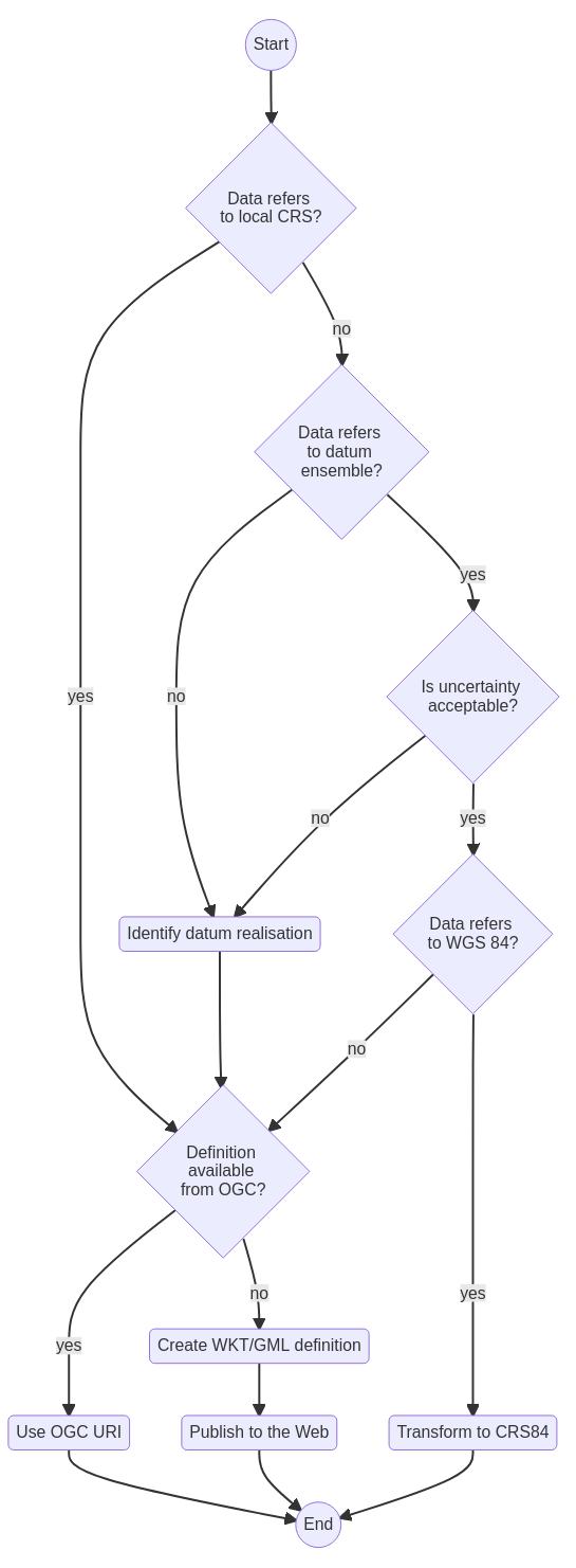
6.6 Raster
By this time you may be wondering why there haven’t been any references yet to raster data in this book. The reason is very simple, that kind of geo-spatial data has never been considered by the W3C, the OGC or any other institution developing standards for the Semantic Web. Raster has all these years remained as the proverbial “elephant in the room”.
This state of affairs does not mean you cannot provide raster data within the Semantic Web. Everything is a resource, and so is a raster. As long as it can be referenced with a URI it may too be referenced from knowledge graphs. The Semantic Web can thus be used for two important roles: convey the semantics of the data stored in the raster and provide its meta-data. The SOSA web ontology (Section 3.5.2) is particularly important in the first of these roles. It is the basis to express concerned environment variables and associated processes. QUDT adds further context on units of measure (Section 3.5.3). Keep in mind that better than using these ontologies directly is to use an existing ontology in the domain. Chapter 9 is fully dedicated to meta-data, there you may read on various useful ontologies. At present the main disadvantage of raster data relative to vector in the Semantic Web is the absence of a processing syntax, like the one GeoSPARQL outlines (Section 6.3).
The reminder of this section briefly reviews modern options for raster provision on the web that fit well with the Semantic Web.
6.6.1 Cloud Optimised GeoTIFF
The Cloud Optimised GeoTIFF (COG) is a community specification for
the provision of raster data on the web. It makes use of the
range parameter in the GET HTTP request to
provide random access to a remote GeoTIFF. Thus a user may request a
particular segment of interest from a large raster with a simple HTTP
request. Since it relies directly on the HTTP protocol, COG dispenses
specific server side software for publication, an HTTP server such as
Apache suffices. The most common use case seems to be the publication of
GeoTIFF files in Amazon’s S3 bucket resources. Although a lightweight
option for segmented raster provision, COG does not allow for in-built
tile caching mechanisms. Therefore it can easily generate an
unmanageable number of requests, especially during remote
visualisation.
At the time of this writing, the OGC is coming towards the eventual approval of COG as a standard. There are however limitations with the original GeoTIFF specification that must be tackled. Prominently is the limited scope of the internal CRS definition in a GeoTIFF, a simple integer number that does not allow the specification of an authority, for instance. COG is not the perfect offer for the Semantic Web but it can still be a useful solution. If on the one hand it is not possible to reference a raster segment with a COG URI, it requires very little work for deployment.
6.6.2 OGC Standards
Canonical mechanisms to access raster maps over the web were long ago
specified by the OGC, especially with the Web Coverage Service (WCS)
(Baumann
2010). Listing 136 provides an example requesting a raster
segment with WCS version 2, limited in Easting and Northing coordinates.
WCS leverages its parameters on the query segment of the URI, making for
long identifiers. But in turn conveys precise raster segments that can
be useful in knowledge graphs. Also worth mentioning is the
DescribeCoverage request that provides meta-data on the
raster.
Listing 136: URI encapsulating a GetCoverage request to a WCS.
https://my-service/maps&
SERVICE=WCS&
VERSION=2.0.1&
REQUEST=GetCoverage&
COVERAGEID=the_raster&
SUBSET=X(4000,8000)&
SUBSET=Y(6000,9000)
WCS and its sibling web services are based on the SOAP/XML specification, which has fallen out of fashion with programmers and modern web technologies. Since 2018 the OGC has been working on a series of new standards for web access to geo-spatial resources based on remote API specifications such as the OpenAPI (Miller et al. 2021) and OData (Chappell 2011). OGC API Coverages is meant to be the modern counterpart to WCS, it has been in development for several year but does not seem to be yet close to become a standard. Issues with the way in which to pass parameters to the service linger. But in parallel the OGC has approved the Environmental Data Retrieval (EDR) API, a simplified specification that does not target raster data per se. However, it proposes a generic data access mechanism that suits raster quite well. Like in WCS, the query segment of the URI is used to pass a myriad of different parameters to the service. Just as Listing 137 exemplifies, this specification can also be used to reference raster resources, their segments and meta-data on the web. Section 8.2 will dive into the coupling of OGC APIs with the Semantic Web in more detail.
Listing 137: URI encapsulating a data request to an EDR API.
http://my-service/api/collections/some-data/area?
  coords=POLYGON((-6.1 50.3,-4.35 51.4,-2.6 51.6,-2.8 50.6,-5.3 49.9,-6.1 50.3))&
  f=GeoTIFF
6.6.3 Discrete Global Grid Systems
The Earth is spherical but maps are flat, a problem as old as Geography itself. Dividing the surface of the plane with squares is a fine approach in small areas, but at the global, regional or even large country scale, distortion rapidly become a challenge. Research in the United States in the late 1980s and early 1990s gave rise to the idea of Discrete Global Grid Systems (DGGS), a trigonometric system for the systematic sub-division of the Earth’s surface with quasi-regular polygons, usually based on its projection on a platonic solid. Even though research has been continuous on this topic, for many years DGGS remained but a curiosity. Until 2016, when Uber adopted a DGGS as the backbone of its internal geo-spatial location, publishing an open-source toolbox along with it20.
Soon after the OGC started work on a DGGS specification, which many hoped to result in some sort of consensus on the trigonometry (or trigonometric principles) for the Earth’s surface sub-division. The result was rather underwhelming, with a meta-standard published instead. However, the past few years work has been conducted on an DGGS API specification for data retrieval and grid querying. While not an off-the-shelf option at the moment, the DGGS concept is increasingly appearing as the future of geo-spatial, providing unequivocal location and subdivision on the whole surface of the Earth, all the while avoiding the distortions associated with map projections.
7 Data Transformation
Up to this point this book has been fairly academic, presenting the abstract elements of the Semantic Web and how they shape digital data. In the process you learnt ontologies, tools and languages that allow you to work with geo-spatial RDF. But here this book tries to answer a more practical and perhaps fundamental question: how to obtain the RDF in the first place? Likely you work with legacy data stored in ancient formats and data stores. Measuring instruments in general do not provide RDF, rather raw data streams that must be processed into usable data.
This chapter presents a few tools and methods that answer the question above. The examples provided span cases in which data may be well structured in a relational database, or exist in simple text files. Data transformation into RDF is a capital step when approaching the Semantic Web. And to perform it well, you must above all understand the semantics of the domain and which ontologies can you use to properly capture it. Hence the late appearence of this chapter.
7.1 Devise a URI structure
Before transforming data into RDF to make it available on the internet, you must first devise an appropriate URI structure. Every non-literal element in a knowledge graph must correspond to a URI, that must be created, or minted, when the RDF is produced. Recall here the introduction to URIs in Section 2.1, URIs are useful even outside the Semantic Web paradigm, as they provide unique identifiers on the WWW to any of your datasets and elements they may contain.
A simple approach is to construct your URIs with three building blocks:
Use a sub-domain of your institutional domain to identify a single project or knowledge graph. E.g.
cycling.my-institute.org.Add a path that starts with the name or identifier of the class to which the data instance belongs. This can be a database table or UML class that matches a class in the target web ontology. E.g.
/landmarksin the Mobility Geography ontology.Complete the path with a number or string that unequivocally identifies the data instance within the class. If you work with relational databases this may be the table primary key. An example:
#zijpenberg.
Listing 138 presents two complete templates for this approach. One
uses the hash (#) character to separate the instance
identifier as a fragment, the second uses the path separator
(/). Both templates are valid, but imply different data
provision options. With the hash character the URI resolves to a
fragment in a document, thus matching the publication of the knowledge
graph in text form, possibly through a simple HTTP server (e.g. Apache).
With the path separator a more sophisticated data provision mechanism is
implied. That will be a topic for Chapter 8.
Listing 138: Templates for URI minting.
http://cycling.my-institute.org/class#identifier

http://cycling.my-institute.org/class/identifier
7.1.1 The Gelderland example
There have been a few examples already in this manuscript of URIs
created for individuals in knowledge graphs. This section revisits the
Gelderland knowledge graph (Section 6.4). This is a small knowledge
graph, published to the web in the form of a text document. Since this
it is just an illustration to the manuscript, the knowledge graph
document is identified a path instead of a sub-domain
(<https://www.linked-sdi.com/gelderland>). And
matching publication as a text document, individual URIs use the hash
character as separator to the identifier
(e.g. #zijpenberg), without distinguishing between classes.
Listing 139 recalls a few of these identifiers in non-abbreviated
form.
Listing 139: Individual URIs in the Gelderland knowledge graph.
https://www.linked-sdi.com/gelderland#radioKotwijk

https://www.linked-sdi.com/gelderland#zevendalseweg

https://www.linked-sdi.com/gelderland#zijpenberg
The Gelderland example is a simple and pragmatic approach to URI minting. The template presented in Listing 138 is a more thorough approach that possibly suits a wider range of cases, but other approaches can certainly be successful. When devising a URI minting mechanism you should take into account at least tow aspects: (i) how it facilitates the transformation of legacy data into RDF, and (ii) how it makes the resulting RDF accessible over the internet.
7.2 From GeoPackage to SPARQL
Recall here the discussion in Section 6.5 regarding coordinates order
with geodetic CRSs. The examples presented in this section with the
GeoPackage format only apply to cartographic CRSs and geodetic CRSs with
swapped coordinates order, such as CRS84. At the current
stage of development GeoPackage (and SpatiaLite in general) cannot be
used with traditional geodesic CRSs such as WGS84 or ITRF89.
7.2.1 SQLite commands
The great thing about the GeoPackage file format is it actually being a small relational database, leveraged on SQLite and Spatialite. Beyond being able to use it in a desktop programme like QGis, or feeding it to a data service software like MapServer, you can interact with it directly with SQL or through an Object-Relation Mapping (ORM) library. That being the simplest path to automation.
To interact with a SQLite database you can start a session directly
at the command line. Listing 140 shows an example, against the
Landmarks.gpkg file21 used previously in
Section 6.4. SQLite informs you the version installed on your system and
presents a new prompt with the sqlite> string. Among
other things, this prompt processes SQL queries.
Listing 140: Starting a SQLite session on a GeoPackage file.
$ sqlite3 Landmarks.gpkg
SQLite version 3.36.0 2021-10-26 10:02:50
Enter ".help" for usage hints.
sqlite>
Before starting to interact with the database you need to load the Spatialite extension (as shown in Listing 141). This extension contains functions and types specific to spatial data that are used even in non-spatial operations, it is always necessary to interact with a GeoPackage database.
Listing 141: Loading the Spatialite extension.
SELECT load_extension("mod_spatialite");The SQLite prompt provides more ways of interaction beyond SQL. For
instance, the command .tables shows the tables present in
the database. Listing 142 shows the output again with the
Landmarks.gpkg file. The Landmarks table
(matching the file name) contains the actual geometries and attributes,
whereas all the others contain internal meta-data for the GeoPackage
format. In a GeoPackage file with more than one geometry table, you can
query the gpkg_contents table to identify them.
Listing 142: Show contents of a SQLite database.
.tables
Landmarks                           gpkg_spatial_ref_sys
gpkg_contents                       gpkg_tile_matrix
gpkg_extensions                     gpkg_tile_matrix_set
gpkg_geometry_columns               rtree_Landmarks_geom
gpkg_metadata                       rtree_Landmarks_geom_node
gpkg_metadata_reference             rtree_Landmarks_geom_parent
gpkg_ogr_contents                   rtree_Landmarks_geom_rowid
Another useful command in the SQLite prompt is .schema,
which lists the SQL code creating a table. Listing 143 exemplifies its
use against the Landmarks table. Using .schema without
providing a target table lists the full SQL underlying all the tables in
the database.
Listing 143: Describe a SQLite table
.schema LandmarksThese simple commands are enough to get you started with
transformations from GeoPackage to RDF. Use the command
.help to get a list of all the commands available in the
SQLilte prompt to know more. Finally, use .exit to
quit.
If you are not so inclined to use the command line to interact with a SQLite database, there is an official graphical user interface for SQLite named DB Browser for SQLite22, although its use is outside the scope of this manuscript.
7.2.2 Obtaining RDF with SQL
The following example makes again use of the
Landmarks.gpkg file to obtain a new RDF instance for each
spatial feature in one go. The outputs will be similar to those
presented in Listing 122 of Section 6.4, then to be gathered in the
Gelderland knowledge graph (gelre: prefix). Starting with
the mob-geo:Landmark instances, there are four to obtain
from the GeoPackage attribute table:
- identifier
- name
- facilities boolean value
For the identifier a string is necessary to append to the
:gelre prefix, to complete a full URI. The
name field in the attribute table can be use for this
purpose, but without spaces and with the first character in lower case
to distinguish the subject as an instance. As with many other database
management systems, SQLite provides a series of string manipulation
functions greatly simplifying this task. SUBSTR obtains the
segment of a string, allowing for their alternative treatment. As its
name implies, REPLACE substitutes characters within a
string, perfect to remove blank spaces. Finally, LOWER can
be used to obtain that first lower case character. These three functions
are combined to obtain a URI for the Landmark individual in line 1 of
Listing 144. The same combination is used to obtain an URI for the
geo:Geometry individual, with the addition of the prefix
Geom.
The name of the spatial feature can be used without manipulation in
the RDF output, the only aspect to be careful with is the language tag.
Finally for facilities boolean there is a peculiarity with
SQLite to be aware of, it does not actually store boolean values, rather
integers. The value 1 stands for true, whereas
0 represents false. Luckily the string
functions provided by SQLite can be applied directly to integers, so it
becomes easy to replace them with strings in the RDF output.
Listing 144 brings all these tasks together in a single SQL query. If
you have not done so yet, start a new SQLite session against the
Landmarks.gpkg file and try this query.
Listing 144: Obtaining Landmark instances from a GeoPackage database with SQL.
SELECT 'gelre:' || LOWER(SUBSTR(name, 1, 1)) || REPLACE(SUBSTR(name, 2, 100), ' ', '') || ' a mob-geo:Landmark ;' || char(10) ||
       '    rdf:label "' || name || '"@en ;' || char(10) ||
       '    geo:hasGeometry gelre:' || LOWER(SUBSTR(name, 1, 1)) || REPLACE(SUBSTR(name, 2, 100), ' ', '') || 'Geom ;' || char(10) ||
       '    mob-geo:facilities "' || REPLACE(REPLACE(facilities, '1', 'true'), '0', 'false') || '"^^xsd:boolean .' || char(10)
  FROM Landmarks;
With the spatial feature encoded as RDF the next step is to obtain a
further individual with the corresponding geometry. The URI was already
obtained in Listing 144, adding the suffix Geom to the
feature URI. The final step is thus the encoding of the WKT literal.
Section 6.4.1 already provided the main elements to obtain a geometry in
the WKT format with the SQLite functions CastAutomagic and
AsWKT. Recall again that these require the Spatialite
extension to be loaded in the SQLite prompt. Listing 145 assembles these
functions to return a Point individual for each feature in
the Landmarks table.
Listing 145: Obtaining Point instances from geometries in the Landmarks vector GeoPackage.
SELECT 'gelre:' || LOWER(SUBSTR(name, 1, 1)) || REPLACE(SUBSTR(name, 2, 100), ' ', '') || 'Geom a geo:Geometry, sf:Point ;' || char(10) ||
       '    geo:asWKT "' || AsWKT(CastAutomagic(geom)) || '"^^geo:wktLiteral .' || char(10)
  FROM Landmarks;
Try now to assemble these individuals together in a Turtle file and
load it to a triple store. Use the abbreviations in Listing 146. Then
you can move to experiment obtaining individuals for the line and
polygon features in the files CyclePaths.gpkg and
NatureAreas.gpkg files23.
Listing 146: URI abbreviations for Landmark features and corresponding geometries
@prefix rdfs:  <http://www.w3.org/2000/01/rdf-schema#> .
@prefix geo: <http://www.opengis.net/ont/geosparql#> .
@prefix sf: <http://www.opengis.net/ont/sf> .
prefix mob-geo: <http://https://www.linked-sdi.com/mobility-geo#> .
@prefix gelre: <http://https://www.linked-sdi.com/gelderland#> .
7.2.3 Going further
The transformation patterns shown above are relatively simple but cover a great deal of circumstances. String manipulation functions are employed to obtain URIs and encode feature properties, spatial functions provide the WKT (or GML in alternative). These patterns can be used against any other spatially enabled database, such as the popular Postgres/PostGIS combination.
If you are comfortable enough with SQL, you can further automate the transformation to RDF with views. If you are not so comfortable, SQL is a worthy investment. It remains one of the most used programming languages in the world, a powerful tool for any data scientist/analyst, even those focused on the Semantic Web.
7.3 tarql
tarql presents a simple proposal: allow for a
CONSTRUCT SPARQL query to be executed against a CSV file,
instead of a triple store. The programme outputs a knowledge graph that
may itself be deployed to a triple store or outright published to the
web. This is a lightweight proposal that can still be very useful,
considering the ubiquitousness of CSV for raw data exchange.
7.3.1 Install
A compressed file with the latest version of tarql can
be obtained from the project releases page 24.
Once the file is decompressed, a new folder is created with the release
number appended, for instance tarql-1.2. The sub-folder
bin contains executables for both Linux and Windows. You
may run the executable directly or install it for wider system use. On
Linux it is common practice to copy the programme folder to
/opt and then create a symbolic link in
/usr/local/bin. Finally try invoking the executable to make
sure it is functioning, as Listing 147 shows.
Listing 147: Simple instructions to install and test run tarql.
$ unzip tarql-1.2.zip
$ sudo mv tarql-1.2 /opt
$ sudo ln -s /opt/tarql-1.2/bin/tarql /usr/local/bin/tarql
$ tarql --help
7.3.2 Use
7.3.2.1 Bicycles and Owners
A simple start is in Listing 148, with a CSV file including some of the information in the Cyclists knowledge graph. It encodes four bicycles, belonging to two different owners plus basic information on weight and brand. These data were already encoded as RDF, but here they serve as an example in a transformation from unstructured data to RDF triples complying with the Mobility ontology.
Transforming these data into RDF with the Mobility ontology implies
the creation of two kinds of instances, some of the type
Owner and others of Bicycle. The query in
Listing 149 preforms this transformation. The CONSTRUCT
clause in the query is pretty standard, yielding a series of triples in
all similar to those in the original Cyclists knowledge graph. It is in
the WHERE clause that magic happens, with the
BIND and URI functions creating new literals
and URIs. The first remarkable aspect to note in this query is the use
of column names in the CSV file as variables, ?Owner,
?Bicycle, ?Brand, etc. tarql
matches every variable with the CSV columns, replacing them with the
corresponding values. For the rest, it is SPARQL at work:
STRLANG assigns language to strings, STRDT
assigns types to literals, plus CONCAT and
LCASE to manipulate strings.
With the contents of Listing 148 saved as Cyclists.csv
and those of Listing 149 as Cyclists.sparql, the programme
can be invoked simply as
tarql Cyclists.sparql Cyclists.csv. The result is presented
to the standard output (STDOUT on Linux) and can easily be
redirected to a file for persistence.
Listing 148: Elements of the Cyclists knowledge graph recorded as an unstructured CSV file.
Owner,Bicycle,Weight,Brand
Machteld,Special,11.3,Isaac
Machteld,K9,13.8,Gazelle
Jan,Tank,10.4,Focus
Jan,Springbok,11.5,Gazelle
Listing 149: SPARQL query transforming the contents of a CSV file into RDF with tarql.
PREFIX rdf: <http://www.w3.org/1999/02/22-rdf-syntax-ns#>
PREFIX rdfs: <http://www.w3.org/2000/01/rdf-schema#>
PREFIX xsd: <http://www.w3.org/2001/XMLSchema#>
PREFIX mob: <https://www.linked-sdi.com/mobility#>

CONSTRUCT
{
    ?uri_owner rdf:type mob:Owner ;
               rdfs:label ?OwnerWithLang .

    ?uri_bicycle rdf:type mob:Bicycle ;
                 rdfs:label ?BicycleWithLang ;
                 mob:weight ?WeightWithType ;
                 mob:brand ?BrandWithLang ;
                 mob:ownedBy ?uri_owner .
}
WHERE
{
    BIND (URI(CONCAT('https://www.linked-sdi.com/cyclists#',
          LCASE(?Owner))) AS ?uri_owner)
    BIND (URI(CONCAT('https://www.linked-sdi.com/cyclists#',
          LCASE(?Bicycle))) AS ?uri_bicycle)
    BIND (STRLANG(?Owner, "en") AS ?OwnerWithLang)
    BIND (STRLANG(?Bicycle, "en") AS ?BicycleWithLang)
    BIND (STRLANG(?Brand, "en") AS ?BrandWithLang)
    BIND (STRDT(?Weight, xsd:decimal) AS ?WeightWithType)
}
7.3.2.2 Remove duplicates
By default tarql generates a triple for each line in the
CSV file. Most likely the data in the CSV is not normalised, and thus
many duplicates result. You can observe this with the instance of the
Owner class above. The tool provides a specific argument to deal with
duplicates: --dedup. It suppresses all duplicate triples up
to a given line in the output. In general you will want to use this
argument with a large enough number to cover all the triples produced.
E.g. tarql --dedup 1000 Cyclists.sparql Cyclist.csv. If
your only intention is to load tarql’s output to a triple
store, you might not need to worry about duplicate triples. Most likely
the software automatically discards the duplicates on load.
7.3.2.3 Landmarks
Listing 150 contains the set of landmarks used previously in Section
6.4, this time encoded as a CSV file lacking semantics. Transforming
this example requires the creation of geo-spatial instances. In first
place the declaration of GeoSPARQL Feature instances, and
then the respective geometries (instances of the Point
class in this case). The query performing this transformation (Listing
151) applies similar patterns to those used in Listing 149. The
URI function again mints new URIs for the resulting RDF
instances. STRDT is now employed to create a new WKT
literal enconding the actual landmark geometry.
Listing 150: The Landmarks in the Gelderland knowledge graph recorded as an unstructured CSV file.
lon,lat,name,facilities
5.81964098736039,52.1734964800341,Radio Kotwijk,"false"
6.02125237622233,52.0284871114981,Posbank,"true"
6.0050321193034,52.0258980219516,Zijpenberg,"false"
5.86709183185877,51.8568380452476,Lentse Warande,"false"
5.91500636067229,51.8248043704151,Berg en Dal,"false"
5.7614399118364,52.0622661566825,Mossel,"true"
Listing 151: SPARQL query transforming the contents of a CSV file into GeoSPARQL with tarql.
PREFIX rdf: <http://www.w3.org/1999/02/22-rdf-syntax-ns#>
PREFIX rdfs: <http://www.w3.org/2000/01/rdf-schema#>
PREFIX geo: <http://www.opengis.net/ont/geosparql#>
PREFIX xsd: <http://www.w3.org/2001/XMLSchema#>
PREFIX mob-geo: <https://www.linked-sdi.com/mobility-geo#>

CONSTRUCT
{
    ?uri_landmark rdf:type mob-geo:Landmark ;
                  rdf:type geo:Feature ;
                  rdfs:label ?NameWithLang ;
                  mob-geo:facilities ?FacilitiesWithType ;
                  geo:hasGeometry ?uri_geo .

    ?uri_geo rdf:type geo:Geometry, sf:Point ;
             geo:asWKT ?geom .
}
WHERE
{
    BIND (URI(CONCAT('https://www.linked-sdi.com/gelderland#',
          LCASE(REPLACE(?name, " ", "")))) AS ?uri_landmark)
    BIND (URI(CONCAT('https://www.linked-sdi.com/gelderland#',
          LCASE(REPLACE(?name, " ", "")), 'Geom')) AS ?uri_geo)
    BIND (STRDT(CONCAT("POINT(", $lon, ", ", $lat, ")"),
          geo:wktLiteral) AS ?geom)
    BIND (STRLANG(?name, "en") AS ?NameWithLang)
    BIND (STRDT(?facilities, xsd:boolean) AS ?FacilitiesWithType)
}
While CSV files may be far more extensive that the small examples showed here, they usually result in similar transformation patterns to RDF. The minting of URIs, redundancy removal and encoding of literals are the most recurrent actions.
7.4 The RML.io tool set
RML.io is a toolset for the generation of knowledge graphs. Its tools automate the creation of RDF from diverse data sources, primarily unstructured tabular data. RML.io comprehends programmes to be used on-line and to be installed on computer systems (Linux, MacIntosh and Windows platforms are supported). The former are useful for prototyping, whereas the latter are meant for actual transformations of large datasets.
7.4.1 The YARRRML syntax
RML.io tools apply data transformations according to a set of rules
recorded in a YAML file. This file must respect a specific syntax, named
YARRRML (Van Assche et al.
2023). This specification defines a number of sections (or
environments) in the YAML file that lay out the structure of the
resulting triples. The first of these sections is named
prefixes and provides the space for the definition of URI
abbreviations, in all similar to the Turtle syntax. Each abbreviation is
encoded as a list item and can be used in the reminder of the YARRRML as
it would be in a Turtle knowledge graph (Listing 152).
Listing 152: YARRML syntax to create triples encoding the weight and owner of bicycles with the Mobility ontology.
prefixes:
 rdf: http://www.w3.org/1999/02/22-rdf-syntax-ns#
 xsd: http://www.w3.org/2001/XMLSchema#
 mob: https://www.linked-sdi.com/mobility#

mappings:
  bicycles:
    sources:
      - ['Cyclists.csv~csv']
    s: https://www.linked-sdi.com/cyclists#$(Bicycle)
    po:
      - [a, mob:Bicycle]
      - [mob:ownedBy, https://www.linked-sdi.com/cyclists#$(Owner)~iri]
      - p: mob:brand
        o:
           value: "$(Brand)"
           datatype: xsd:string
      - p: mob:weight
        o:
           value: "$(Weight)"
           datatype: xsd:decimal
Next comes the mappings section, where the actual
transformations are encoded. This section is to be populated with
sub-sections, one for each individual class (or type) necessary in the
output RDF. For instance, if the transformation must produce triples for
owners and bicycles, then a sub-suction for each is necessary. The name
of these subject sub-sections is arbitrarily chosen by the user. For
each subject class sub-section at least one data source needs to be
specified in the sources section. The source can be
declared within square brackets (i.e. a YAML collection), providing a
path to a file followed by a tilde and then a type. The sources section
can be more intricate, as YARRRML supports a wide range of different
data sources 25, including flat tables, databases
and Web APIs.
The following sub-section for the class declares the subject and has
the simple name of s. Its purpose is to define the URI
structure for the instances of the class. In principle this is also the
first element that makes reference to the contents of the source file.
In the case of a CSV file the column names are used. They are invoked
using the dollar character ($), with the column name within
parenthesis. The practical result is the generation of an individual
element (subject in this case) for each distinct value found in the
source column.
With the subject defined, triples can be completed with predicates
and objects in the po sub-section. This sub-section is
itself composed by a list, whose items comprise a pair: predicate (item
p) and object (item o). The predicate is
encoded as a URI in a similar way to the subject, using abbreviations if
necessary. As for the object, it can be decomposed further into a
value and a datatype to accommodate literals.
The example in Listing 152 creates triples for the Bicycle class
subject, using the Bicycle column in the source to generate
subject URIs. The source column Weight is used to complete
triples declaring the weight of the bicycle.
The encoding of the predicates and objects can be shortened, instead of discriminating value and data type, they can be instead expressed as elements of a collection. This formulation is useful when the object is itself a URI. Note how in Listing 152 the tilde is used again, to indicate the object type, a URI in this case.
This was just a brief introduction to the YARRRML syntax. It goes far deeper, even allowing for some functional programming. While the guidelines in this document make enough of a start to automated RDF generation, the YARRML manual (Van Assche et al. 2023) is indispensable to take full advantage of the RML tool set.
7.4.2 Matey
The simplest way to start using RML.io is through the Matey online user interface 26. It is an excellent prototyping tool and will help you getting acquainted with the YARRRML syntax.
The standard view of Matey has 4 sections:
- data input;
- definition of YARRRML rules;
- RDF output display;
- visualisation of RML.io rules exported from YARRRML.
There are various examples available to guide you through the basics of YARRRML and RML. Take some time to experiment with these examples, try modifying the output, or even to create further transformation rules.
Eventually you will find the limitations of Matey, while convenient for prototyping, it does not scale for large datasets or to process a large number of source files. For that you need to use the command line interface.
7.4.3 Install
Using RML.io in your system requires two programmes, a parser for the
YARRRML syntax (yarrrml-parser) and a transformer that
converts tabular data to RDF (rmlmapper). Installation is
exemplified in Listing 153. yarrrml-parser is installed
with npm, whereas rmlmapper is a Java
programme, that can be downloaded directly from the project GitHub page
27. rmlmapper is run with
the Java Runtime Environment, and might be useful to create a shortcut
to invoke it with a simple command. How to do this depends on your
system and is beyond the scope of this document.
Listing 153: Basic instructions to install rmlmapper.
npm i -g @rmlio/yarrrml-parser

wget https://github.com/RMLio/rmlmapper-java/releases/download/v6.1.3/rmlmapper-6.1.3-r367-all.jar

java -jar rmlmapper-6.1.3-r367-all.jar
7.4.4 How to use
For this example the CSV files in Listing 148 and Listing 150 are used again. The goal is the same, to reproduce, in total or in part, the triples originally created for the Cyclists and Gelderland knowledge graphs.
7.4.4.1 Bicycles
The simplest place to start is with the bicycles. There are three essential elements to generate for each bicycle:
- a new URI for the bicycle;
- the declaration of the new bicycle as an instance of the class
Bicycle; - the association with the respective owner;
- the bicycle brand;
- the bicycle weight.
The contents of Listing 152 encode this transformation. Save it to a
file with a suggestive name like Cyclists.yarrrml. To
perform the actual transformation you must first apply
yarrrml-parser to create the RML transformation file and
then use rmlmapper to obtain the actual knowledge graph. By
default rmlmapper creates a Turtle file that is printed to
the standard output (STDOUT). You can use the parameters -o
to redirect output to a text file and -s to select an
alternative serialisation syntax.
Listing 154: Basic transformation to Turtle with rmlmapper.
yarrrml-parser -i Cyclists.yarrrml -o Cyclists.rml.ttl

rmlmapper -s turtle -m Cyclists.rml.ttl
7.4.4.2 Landmarks
For a geo-spatial example the CSV file in Listing 150 is used again. The appropriate GeoSPARQL instances must be created in this transformation, namely:
- Declaration of the landmark as an instance of the class
geo:Feature; - Creation of a
geo:Geometryinstance to host the actual geo-spatial information; - A literal of the type
geo:wktLiteralorgeo:gmlLiteralto encode the geometry.
The complete transformation is gathered in Listing 155. It shows the
inclusion of two different classes in the same transformation. Note how
the Feature instance is associated with the geometry using
the geo:hasGeometry object property. Also important is the
creation of the WKT literal, as it requires a verbose declaration of the
object to make the type explicit.
Listing 155: YARRML syntax to create triples encoding landmarks with the Mobility ontology.
prefixes:
 xsd: http://www.w3.org/2001/XMLSchema#
 geo: http://www.opengis.net/ont/geosparql#
 mob-geo: https://www.linked-sdi.com/mobility-geo#
 gelderland: https://www.linked-sdi.com/gelderland#

mappings:
  landmark:
    sources:
      - ['Landmarks.csv~csv']
    s: gelderland:$(name)
    po:
      - [a, mob-geo:Landmark]
      - [a, geo:Feature]
      - [geo:hasGeometry, gelderland:$(name)_geo~iri]
      - p: mob-geo:facilities
        o:
           value: "$(facilities)"
           datatype: xsd:boolean

  geometry:
    sources:
      - ['Landmarks.csv~csv']
    s: gelderland:$(name)_geo
    po:
      - [a, geo:Geometry]
      - p: geo:asWKT
        o:
           value: "POINT($(lon) $(lat))"
           datatype: geo:wktLiteral
8 Data Provision
The interaction with RDF data through a SPARQL end-point is one of capital aspects of the Semantic Web, be it for the search capabilities it allows, but also as a fundamental mechanism to data federation. The same reasoning also applies to geo-spatial data, but other forms of RDF provision are becoming relevant. This chapter reviews methods of data provision that simplify data access and browsing to human users. But most importantly, this chapter presents how state-of-the-art OGC data retrieval standards are coalescing with geo-spatial RDF. This is therefore a key segment of this book, in which you will find the most cutting edge (and therefore prone to update) information.
8.1 Virtuoso Facets
Besides all the possibilities it provides as a triple store, Virtuoso also makes available an RDF specific perspective focused on human access to knowledge graphs. This feature is termed Facets and within the open source realm is unique to Virtuoso. As you will learn in this chapter, it is a data provision that can greatly facilitate a first contact with RDF to less sophisticated users, and may also play an instructional role to new comers in the Semantic Web.
8.1.1 Installation and configuration
The Facets perspective is not installed by default in Virtuoso, but the additional packages it requires are straightforward to install. The Virtuoso software largely does the job by itself. These instructions assume you already have a running Virtuoso instance on your system or otherwise at your disposal, as Section 4.1.2 detailed. Access Virtuoso on the web browser and log on to the Conductor page. Once in navigate to the System Admin tab and then to the Packages sub-tab. Virtuoso lists in a table a series of software packages that are installed or may be installed (Figure 30). The packages currently installed report an installed version number and an Unistall action.
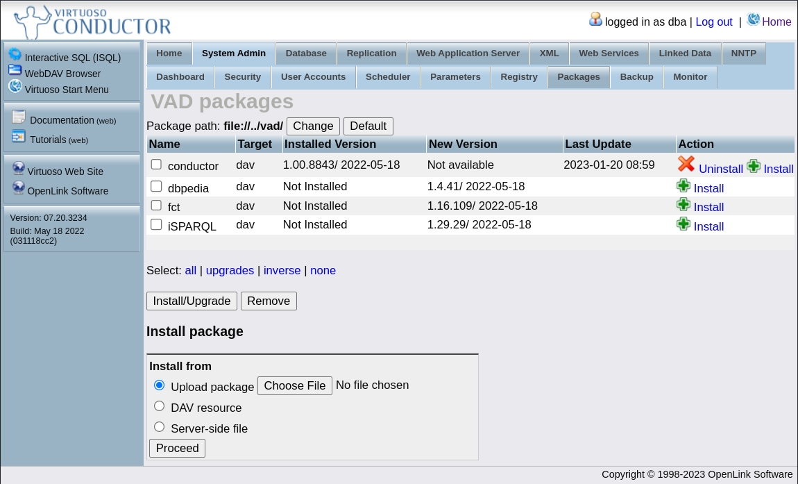
The package corresponding to the Facets perspective is identified with the short name fct. To start its installation you only need to click on the Install action in that row. This takes you to a confirmation page enumerating risks to be aware of when performing this action (Figure 31). Unless you are running an instance with very large knowledge graphs and busy with many requests there is no reason to expect anything to go wrong. The only possible nuisance is an interruption to all interactions with the server, therefore something to be aware of in production. Ideally, a server should go into the production already with all necessary packages installed. After clicking the Proceed button Conductor informs on the Facets version it installed (Figure 32). In this dialogue you may click the Back to Packages button and confirm in the table that Facets is indeed installed.
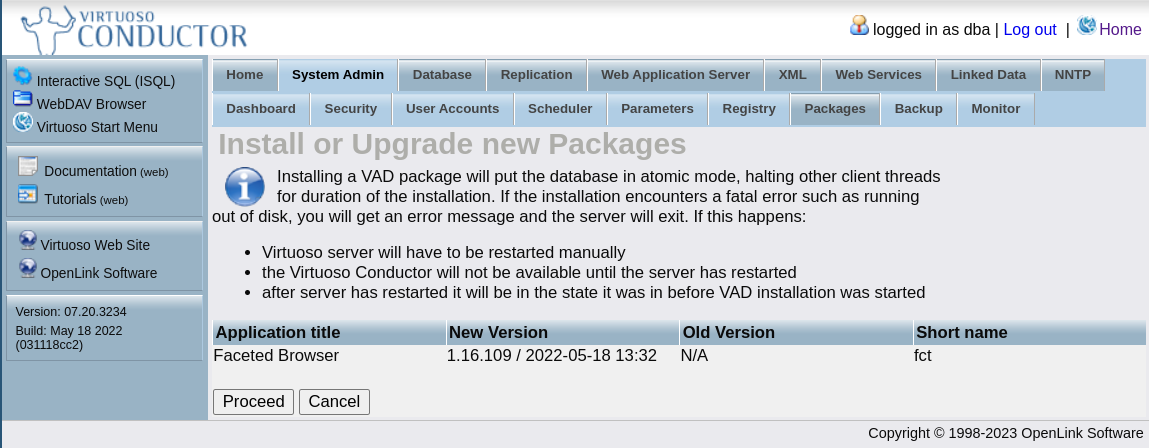
The required software is installed, but Virtuoso still needs to
create the text indexes that support search across all knowledge graphs.
This action is performed in the interactive isql console.
Follow the instructions in Section 4.1.2 if necessary and run the
commands in Listing 156. But that is not all, Facets also uses lookup
tables for labels and URIs to further facilitate search. These are built
with the commands in Listing 157. Whereas the text indexes only need to
be created once, the look-up tables should be regularly updated, again
with Listing 157.
Listing 156: Commands to create the text indexes used by the search function in the Virtuoso Facets perspective.
RDF_OBJ_FT_RULE_ADD (null, null, 'All');
VT_INC_INDEX_DB_DBA_RDF_OBJ ();
Listing 157: Commands to create the look-up tables used by the search function in the Virtuoso Facets perspective.
urilbl_ac_init_db();
s_rank();
8.1.2 The Facets user interface
Facets is now ready to use. Return to the Virtuoso home page, log out
from Conductor if necessary and use the Home button in the top
right. Click on the Faceted Browser button, the browser then
navigates to the /fct path, with the setup given in Section
4.1.2 the full path will be http:0.0.0.0:8890/fct. A home
page is displayed, showing a free text search (Figure 33). Facets
searches across all knowledge graphs for any string literal containing
the text provided. Assuming the Cyclists knowledge graph is loaded in
this Virtuoso instance, you can search for one of the bicycles imagined
in Chapter 3. Type “Slippery” and click Search, a results page
is then presented where you should find the resource corresponding to
that bicycle. Click now on the “Slippery” URI, Facets then takes to what
it calls the entity page for this resource (Figure 34). Take some time
to observe all the information Facets presents, it portrays all triples
having the “Slippery” bicycle as object, one per line. Predicates and
non-literal subjects are portrayed as web links, but if you click them,
Facets presents the corresponding entity page.
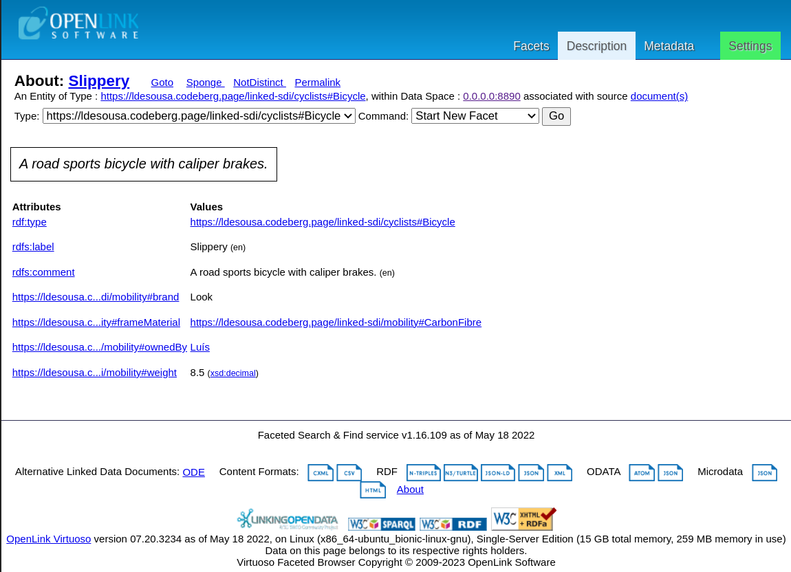
Click now on the “Luís” web link, the subject of the
ownedBy predicate. In this new entity page you are also
presented with the triples having the “Luís” instance as subject, in
this case they represent all the bicycles owned by “Luís” in a specific
row with the formulation “is … of …” (Figure 35). Like this you can
navigate back and forth between bicycles and owner. The denser a
knowledge graph is the more immersive this navigation becomes. And thus
you can observe the power of Facets, conveying the graph-like (or
linked-like) nature of RDF in an expressive way. Back in the Facets home
page you can explore the Labels and URI tabs that
provide for more directed searches, these may be handy with large
knowledge graphs.
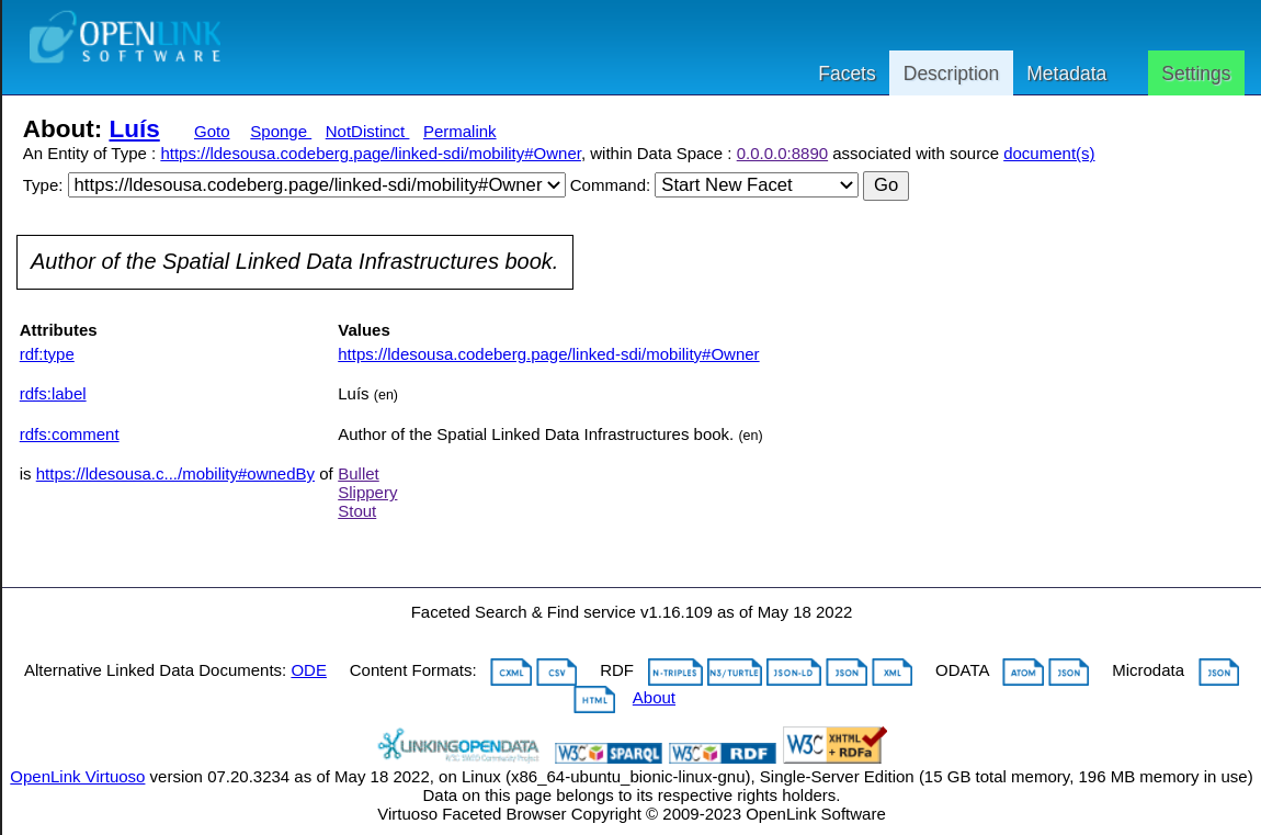
8.2 OGC API Features with Prez
8.2.1 Intro
As Section 1.2.2 exposed, joint work between the OGC and the W3C raised a number of issues with the traditional approaches to SDIs and the publication of geo-spatial data on the web. This was one of the elements triggering a paradigm shift at the OGC, towards a develop first, specify later process. With it came the transition to developer friendly ReST APIs, based on the Open API specification.
While the OGC has largely kept at bay from the Semantic Web (apart from the lone GeoSPARQL initiative) in fact this drive towards REsTful APIs meant a decisive step towards the Linked Data paradigm. Take for instance the Features API, it opened up the response document format to modern specifications, particularly JSON. JSON-LD being a specialisation of the latter the door was left wide open for a direct bridge to the Semantic Web.
An early attempt within the reference pygeoapi project28 was not able to overcome lingering (and unwarranted) scepticism of the Semantic Web. However, the urge among Australian institutions to lead web technology development, eventually resulted in the Prez project. Currently in development by Surround Australia, Prez is able to serve geo-spatial knowledge graphs from any triple store exposing a SPARQL endpoint, serving them through a Features API. Therefore, any client software able to interact with an OGC Features API can access geo-spatial triples.
This section provides an introduction to Prez. It explains the meta-data necessary to render a knowledge graph usable by Prez and the basic setup of the software.
8.2.2 OGCLDAPI Profile
The OGC API Features is underpinned on the constructs of Collection and Feature, meeting familiar concepts found in other OGC specifications, notably in GeoSPARQL itself. However, to meet all the requirements and functionalities of the API specification the data and object properties specified in GeoSPARQL are not sufficient. To address that gap Surround Australia specified its own OWL Profile, named OGC Linked Data API Profile (ogcldapi profile for short), adding a number of requirements to a geo-spatial knowledge graph bound to be served by Prez (J. Car Nicholas 2021). An OWL Profile is an abstract ontology specification prescribing a particular structure to be implemented by a concrete ontology (or directly by a knowledge graph).
The ogcldapi profile specifies requirements demanding the presence of individuals from three different class in a compliant knowledge graph:
dcat:Dataset: a concept extraneous to GeoSPARQL that serves the purpose of gathering different Feature Collections under a single umbrella. It allows Prez to distinguish which collections to serve from the source triple store. You may consider this class as equivalent to the broad concept of geo-spatial knowledge graph. You can read more on the DCAT ontology in Section 9.1geo:FeatureCollection: a series of spatial features related to each other in some way. For instance a set of buildings with respective geometries, or a collection of way points surveyed with a GPS receiver. As seen in Section 6.2,FeatureCollectioncan be regarded as a geo-spatial layer, but it goes well beyond that.geo:Feature: the familiar concept of a geo-spatial geometry with associated information (attributes in traditional GIS).
The sub-sections below break down the individual requirements for each of these classes.
8.2.2.1
dcat:Dataset
Each
Datasetindividual must have one and only one English title which is an English text literal, indicated using thedcterms:titlepredicate.Each
Datasetindividual must have one and only one English description which is an English text literal, indicated using thedcterms:descriptionpredicate.Each
Datasetindividual must have one and only one identifier, anxsd:tokenliteral, indicated using thedcterms:identifierpredicate. This identifier must be unique within the Dataset it is part of.Each
FeatureCollectionindividual that is part of dataset must be referenced from the later using therdfs:memberpredicate.A Dataset may indicate a Bounding Box geometry with a
geo:boundingBoxpredicate
8.2.2.2
geo:FeatureCollection
Each
FeatureCollectionindividual must have one and only one English title which is an English text literal, indicated using thedcterms:titlepredicate.Each
FeatureCollectionindividual must have one and only one English description which is an English text literal, indicated using thedcterms:descriptionpredicate.Each
FeatureCollectionindividual must have one and only one identifier, anxsd:tokenliteral, indicated using thedcterms:identifierpredicate. This identifier must be unique within the Dataset it is part of.Each
Featureindividual that is part of the feature collection must be referenced from the latter using therdfs:memberpredicate.A
FeatureCollectionindividual may indicate a Bounding Box geometry with ageo:boundingBoxpredicate
8.2.2.3
geo:Feature
Each
Featureindividual must have one and only one identifier, anxsd:tokenliteral, indicated using thedcterms:identifierpredicate. This identifier must be unique within the dataset it is part of.Each
Featureindividual must indicate that it has at least onegeo:Geometryindividual with use of thegeo:hasGeometrypredicate.
The token individuals are somewhat of a contraption, considering that the URI of an individual is already a unique identifier. It is however understandable the need for shorthand references to individuals in the programme. Apart from the token the other requirements are largely straightforward and possibly already part of a given geo-spatial knowledge graph.
8.2.3 Automation
The requirements set by the ogcldapi profile are not that
demanding, and it is possible your geo-spatial knowledge graph(s)
already meet some of them. For instance, in the Gelderland graph
introduced in Section 6.4, geo:FeatureCollection
individuals could already have been already introduced for internal
organisation. Still, you most likely need to add further triples to
fully comply with the profile. If the graph is extensive this task is
too expensive to perform manually and must be automated in some way.
Here again you can make full use of SPARQL. Using INSERT
queries all the necessary compliance triples can be added without much
effort. Starting again with the Gelderland geo-spatial dataset, this
sub-section walks you through the key queries. The first element to add
is the Dataset instance, the query in Listing 158 provides
the basic elements, yet without automation. Note how the
GRAPH clause is used to restrict the scope of the
query.
Listing 158: SPARQL query adding a new Dataset instance to the Gelderland knowledge graph.
PREFIX gelre: <https://www.linked-sdi.com/gelderland#>
PREFIX xsd: <http://www.w3.org/2001/XMLSchema#>
PREFIX rdfs:  <http://www.w3.org/2000/01/rdf-schema#>
PREFIX dcterms: <http://purl.org/dc/terms/>
PREFIX dcat: <http://www.w3.org/ns/dcat#>

INSERT
{
    GRAPH <https://www.linked-sdi.com/gelderland#> {
        gelre:dset a dcat:Dataset ;
            dcterms:title "Cycling in Gelderland"@en ;
            dcterms:description "Spatial features of interest to
                                 cyclists in Gelderland"@en ;
            dcterms:identifier "Gelre"^^xsd:token .
    }
}
Since the Gelderland knowledge graph does not have feature collections it is necessary to add some. One would be enough, but since there are three distinctive classes of spatial features (landmarks, cycle paths and nature areas), it is wise to create a collection for each of those. Listing 159 shows a query creating the feature collection for landmarks.
Listing 159: SPARQL query adding a new feature collection for Landmark instances.
PREFIX gelre: <https://www.linked-sdi.com/gelderland#>
PREFIX xsd: <http://www.w3.org/2001/XMLSchema#>
PREFIX rdfs:  <http://www.w3.org/2000/01/rdf-schema#>
PREFIX dcterms: <http://purl.org/dc/terms/>
PREFIX dcat: <http://www.w3.org/ns/dcat#>

INSERT
{
    GRAPH <https://www.linked-sdi.com/gelderland#> {
        gelre:Landmarks a geo:FeatureCollection ;
            dcterms:title "Landmarks in Gelderland"@en ;
            dcterms:description "Landmarks interesting to visit
                                 by bicycle in Gelderland"@en ;
            dcterms:identifier "Landmarks"^^xsd:token .
    }
}
So far pretty straightforward queries, but now it is necessary to
link the various individuals with the rdfs:member
predicate. Enter the WHERE clause to the
INSERT query. The former is used to identify all the
feature collections that must be referenced from the
Dataset instance. Note again in Listing 160 the scope
limitation with the GRAPH clause, both within the
INSERT and WHERE clauses. Without it all
feature collections in the triple store would be associated with the
gelre:dset individual. In Listing 161 a similar example is
given associating all features of type Landmark with the
Landmarks feature collection.
Listing 160: SPARQL query linking the dataset with feature collections.
PREFIX gelre: <https://www.linked-sdi.com/gelderland#>
PREFIX rdfs:  <http://www.w3.org/2000/01/rdf-schema#>
PREFIX geo: <http://www.opengis.net/ont/geosparql#>

INSERT
{
    GRAPH <https://www.linked-sdi.com/gelderland#> {
        gelre:dset rdfs:member ?coll .
    }
}
WHERE {
    GRAPH <https://www.linked-sdi.com/gelderland#> {
        ?coll a geo:FeatureCollection .
    }
}
Listing 161: SPARQL query linking the `Landmarks` with its spatial features.
PREFIX gelre: <https://www.linked-sdi.com/gelderland#>
PREFIX rdfs:  <http://www.w3.org/2000/01/rdf-schema#>
PREFIX geo: <http://www.opengis.net/ont/geosparql#>

INSERT
{
    GRAPH <https://www.linked-sdi.com/gelderland#> {
        gelre:Landmarks rdfs:member ?mark .
    }
}
WHERE {
    GRAPH <https://www.linked-sdi.com/gelderland#> {
        ?mark a gelre:Landmark .
    }
}
On to the trickiest bit: automatically create tokens for each
individual. The strategy here is the same as before, an
INSERT query including a WHERE clause
returning all individuals that need a token, plus the token itself.
Making it simple, the token to apply will be the fragment section of the
individual URI. E.g. for the individual with the URI
<https://www.linked-sdi.com/gelderland#mossel> the
token to apply is mossel. The magic happens in the
BIND function in Listing 162. The function
STRAFTER does the magic, returning the remainder of an
input string given a prefix to remove. Since these inputs are originally
URIs, the STR function is used to transform them into
strings. Finally the output of STRAFTER must be transformed
into the xsd:token literal type, as required by
ocgldapi profile. That is the role of the STRDT
function.
Listing 162: SPARQL query adding tokens to spatial features of type `Landmark`.
PREFIX gelre: <https://www.linked-sdi.com/gelderland#>
PREFIX xsd: <http://www.w3.org/2001/XMLSchema#>
PREFIX dcterms: <http://purl.org/dc/terms/>

INSERT
{
    GRAPH <https://www.linked-sdi.com/gelderland#> {
        ?feat dcterms:identifier ?token .
    }
}
WHERE {
    GRAPH <https://www.linked-sdi.com/gelderland#> {
        ?feat a gelre:Landmark .
        BIND (STRDT(STRAFTER( STR(?feat),
                              STR(gelre:)), xsd:token) AS ?token)
    }
}
And that should be about all you need to make a knowledge graph
conforming to the ogcldapi profile. Try now to apply queries
like those above on the Gelderland knowledge graph to make it fully
usable by Prez. The result should be similar to that in the file
GelderlandOCGAPI.ttl, provided with the web version of this
manuscript 29.
8.2.4 Setting up Prez
Prez is still a relatively new software, with a good deal of polishing necessary for a fully seamless user experience. Albeit somewhat agricultural, the set-up is not at all challenging and can be completed in a matter of minutes. In fact applying the ogcldapi profile should be the most time consuming task.
Start by checking out the Prez repository from GitHub, as Listing 163
exemplifies. Then create a new Python virtual environment and install
the dependencies. This can be done either with pip or
poetry, the latter being the recommended practice.
Listing 163: Basic installation instructions for Prez.
$ git clone git clone git@github.com:surroundaustralia/Prez.git

$ cd Prez

$ python3 -m virtual env

$ source env/bin/activate

$ pip install poetry

$ poetry install
With the dependencies installed Prez is now ready to run. However it
needs to know the coordinates to the SPARQL end-point serving the
geo-spatial knowledge graph. This information is set up with the
environment variable SPACEPREZ_SPARQL_ENDPOINT, indicating
the URL to the SPARQL end-point. If you are using Virtuoso in your local
system this URL is http://localhost:8890/sparql. While a
Python configuration file would be preferable, this schema is
functional. Prez is well more than a API Features server, also exposing
services providing other kinds of knowledge graphs. Those are not
covered in this manuscript, just be aware that extra environment
variables are required for those services.
To start the programme proper it is all a matter of executing the
app.py file residing in the prez folder. It
logs activity directly to the command line, therefore you might wish to
re-direct that to a file. In Listing 164 you can find a convenient Bash
script encapsulating this set-up. Note how the logs are redirected to
the file prez/prez.log.
Listing 164: Bash script encapsulating the start up of Prez.
#!/bin/bash

export VOCPREZ_SPARQL_ENDPOINT="http://vocs.my-server/sparql"
export SPACEPREZ_SPARQL_ENDPOINT="http://geo.my-server/sparql"
export TIMEPREZ_SPARQL_ENDPOINT="http://time.my-server/sparql"
export CATPREZ_SPARQL_ENDPOINT="http://cats.my-server/sparql"

source env/bin/activate

cd prez

nohup python3 app.py > prez.log 2>&1 &
Prez will expose its services and web interface on port 8000. At the
time of this writing this port number is hard coded and cannot be
configured. However, if you wish to modify it you may directly edit the
prez/app.py file (search for the method
uvicorn.run).
8.2.5 Containerised deployment
Surround Australia also makes docker images available for convenient deployment. Especially with micro-services platforms in mind. The images available take care of all the necessary software dependencies and expedites the TCP/UDP port attribution. Declaring the source SPARQL end-points with environment variables is thus all that is left to do.
While docker itself provides mechanisms to set up environmental
variables for individual containers, a more thorough configuration can
be achieved with a docker-compose file. In Listing 165 you have a
straightforward example. It references the latest image provided by
Surround Australia, maps port 8000 to a less common port and declares
the environment variables. If you use a docker-compose file as this one
in a development environment, you will possibly be referring to a triple
store run by a software like Fuseki or Virtuoso. In such case use your
system’s IP address 30 to access it from the container,
e.g. http://192.168.178.150:8890/sparql.
Listing 165: Example of a docker-compose file for Prez.
version: '3.3'

services:
  prez:
    image: surroundaustralia/prez:latest

    container_name: prez

    ports:
      - 8990:8000

    environment:
      - VOCPREZ_SPARQL_ENDPOINT=http://vocs.my-server:8890/sparql
      - SPACEPREZ_SPARQL_ENDPOINT=http://geo.my-server:8890/sparql
      - TIMEPREZ_SPARQL_ENDPOINT=http://time.my-server:8890/sparql
      - CATPREZ_SPARQL_ENDPOINT=http://cats.my-server:8890/sparql
8.2.6 The Prez web interface
If direct your internet browser to the port used by Prez you will be
presented with a rich graphical web interface (Figure 36). The term
“Default” is used throughout to indicate this is still a development
instance. For a deployment in production you (or someone in your team
with such competences) are expected to edit the “look and feel” of the
interface. This is made manipulating the assets in the folders
prez/static and prez/templates. The web
interface presents the various services provided by Prez, beyond the
spatial vertent there are also vocabularies, time-series and
meta-data.
Use the menus to navigate to the Datasets list, clicking on the
SpacePrez tab and then Datasets. This page lists all
the instances of the DCAT Dataset class found in the SPARQL
endpoint set up for SpacePrez with the environment variables (e.g.
Figure 165). In Figure 37 Prez list the “Floods” dataset, a test
knowledge graph distributed with Prez. If you then click on red
Collections button for the “Floods” item Prez takes you to the
list of FeatureCollections instances associated with the
“Floods” dataset. In this case there is only one, the “Hawkesbury Flood
2021”, as Figure 38 shows. Similarly, by clicking on the red
Features button for the collection item, Prez takes you to a
list of all associated instances of the GeoSPARQL Feature
class (Figure 39). Now each item of the list is clickable, leading to an
expressive web page listing all data and object properties associated
with the feature. The associated GeoSPARQL geometry is nicely portrayed
in a web map, as Figure 40 shows. At the time of writing only geometries
encoded with the CRS84 CRS can be portrayed.
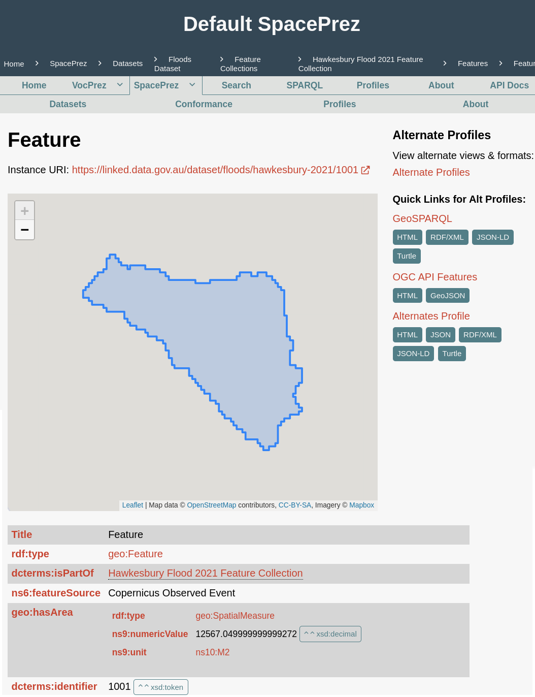
Prez itself provides a SPARQL endpoint, accessible from anywhere in the interface by clicking on the respective tab. This endpoint may appear redundant with the original RDF endpoint, but actually allows to elegantly insulate the latter from remote access if necessary. And following modern conventions, Prez automatically creates a graphical user interface in HTML with the Swagger technology (S. Software 2023). The Swagger graphical interface is accessible from anywhere in the Prez interface through the API Docs tab. Figure 41 shows the segment of the Swagger interface interacting with the OGC API Feature services.
9 Meta-data
“Data is useless without meta-data”. You possibly have heard this adage before, or one of its many variations. This is true also of the Semantic Web, and thus this dedicated chapter. However, it is important to acknowledge the somewhat different role it plays in this context. Meta-data for non-semantic datasets often concerns information such as units of measure, environmental variables or language. That is by and large semantics itself. In fact the traditional meta-data in the geo-spatial world is primarily used as a vehicle to add semantics to datasets that lack it by nature. A CSV file is a good example (as explored in Section 1.1), but so is a raster file or even a portable relational database. Naturally, meta-data does not have the same role with a geo-spatial knowledge graph.
In the Semantic Web meta-data is still important, but primarily to identify the individuals and institutions responsible for knowledge graphs, and elements such as access rights and usage licences. And of course, meta-data is a further means to link related resources together and to third resources of relevance. In this chapter three useful meta-data web ontologies are reviewed: the popular Dublin Core Terms, DCAT for data resources and vCard for individuals and organisations. The chapters closes with a small example covering the knowledge graphs illustrating this manuscript.
9.1 DCAT
The Data Catalog Vocabulary (DCAT) (Albertoni et al. 2020) is the de facto meta-data standard for the Semantic Web. It has been under continuous development by the W3C for over a decade, and is currently published as a recommendation. Its main purpose is to identify data resources in a semantically congruent way. The DCAT ontology links to other meta-data relevant ontologies and is in turn used at large by ontologies meant to standardise meta-data encoding. In particular predicates from Dublin Core meta-data terms ontology are widely used as data and object properties in DCAT classes. Classes from the FOAF and VCard ontologies are in their turn often used as ranges of object properties. In many cases the ranges of object properties are just recommendations, leaving their use open. Whereas developed with the Semantic Web in mind, DCAT is not by any means restricted to represent meta-data of knowledge graphs. In fact at its core is the concept of multiple representations for the same data.
The base URI for the DCAT ontology is
http://www.w3.org/ns/dcat#, usually abbreviated to
dcat:. Figure 42 provides a general overview of the classes
specified in DCAT and their relationships, the following sections
provide details on each.
9.1.1 Resource
In DCAT every concrete thing is a Resource, a super
class that bundles together common data properties and facilitates the
specification of object properties. The three main concrete classes in
DCAT: Dataset, DataService and
Catalog are all sub-classes of Resource. Even
though the concept of abstract class does not exist OWL,
Resource is meant as such, meaning that in your meta-data
there should be no direct instances of this class.
From the long list of data properties specified for the
Resource class the following can be highlighted:
contactPoint: contact person or institution responsible for the resource. Recommended range:vcard:Kind.keyword: a literal describing the resource. Ideally a single word, the smaller the keyword, the likelier it will match other resources.landingPage: a web page providing access to the resource through a web browser. Range:foaf:Document.accessRights: indicates who has access to the resource and under which conditions. Range:dcterms:RightsStatement.creator: Identifies the entity responsible for producing the resource. The recommended range isfoaf:Agent, but in some circumstance it might be better used with VCard.dcterms:description: a literal describing the resource in some detail, without restrictions to length.dcterms:identifier: a literal identifying the resource within a certain context. It does not replace the resource URI, but can be useful within a service or a catalogue.dcterms:license: legal document determining conditions under which the resource is made available. Mostly relevant for open access resources. Range:dcterms:LicenseDocument.dcterms:title: a literal providing a short, human readable name for the resource.
9.1.2 Dataset
As its name implies, this class represents a collection of data, but with the restriction of being published or curated by a single entity. It can be thought of as a knowledge graph, or the segment of a knowledge graph, administered by a single institution or individual. The same dataset may be encoded and/or presented in different ways, and even be available from different locations. Relevant properties are summarised below:
distribution: a representation of a dataset. Range:Distribution.spatialResolutionMeters: meant primarilly for images or raster grids, but can also be used to characterise positional accuracy in vector datasets. Range:xsd:decimal.temporalResolution: minimum time interval represented in the dataset. Range:xsd:duration.dcterms:spatial: the spatial extent covered by the dataset. Range:dcterms:Location, representing an area or a named place.dcterms:temporal: the time period covered by the dataset. Range:dcterms:PeriodOfTime.prov:wasGeneratedBy: identifies the activity that generated the dataset. As specified by the PROV ontology, the range isprov:Activityand the domainprov:Entity. Thus to use this object property the concerned dataset must be declared as of typeprov:Entity.
9.1.3 DataService
DCAT not only represents data resources but also the means to
retrieve them, that being the role of the DataService
class. It captures operations that provide access to datasets and also
data processing services. A DataService instance in general corresponds
to a service point accessible on the internet. The specific properties
are:
servesDataset: withDataServiceas domain andDatasetas range, it informs on the datasets provided by a particular service.endpointURL: service location on the internet. Range:rdfs:Resource.endpointDescription: location of a document describing the service, respective operations and parameters. May be a machine readable document. Range:rdfs:Resource.
9.1.4
Distribution
DCAT recognises that each dataset may be represented in different
ways, therefore the Distribution class describes various
such representations for a dataset. For example, a geo-spatial knowledge
graph may also be encoded as a GML document, but is in essence the same
dataset. Also within the same concept of dataset fit representations of
different level of detail, e.g. different spatial or temporal
resolutions. Relevant properties:
accessService: relates the distribution instance to a data service. Range:dcat:DataService.accessURL: location of a resource providing access to this representation of the dataset, a SPARQL end-point is an example. Range:rdfs:Resource.compressFormat: declares a compression format in case the distribution corresponds to a compressed representation of the dataset. Range:dcterms:MediaType.downloadURL: URL of a downloadable file corresponding to this representation of the dataset. Range:rdfs:Resource.mediaType: media type of this dataset representation, according to the IANA list of Media Types (Melnikov, Miller, and Kucherawy 2023). Range:dcterms:MediaType.packageFormat: packaging format of the distribution, in case the dataset is represented as a bundle of multiple files. Range:dcterms:MediaType.spatialResolutionInMeters: same function as inDataset.temporalResultion: same function as inDataset.format: file format of the distribution, in case it is represented as such. Range:dcterms:MediaTypeOrExtent.title: same function as inDataset.accessRights: same function as inDataset.license: same function as inDataset.
9.1.5 Catalog
A set of meta-data about resources that are somehow related, managed
together or available from a single location, may be aggregated within a
meta-data catalogue (the Catalog class). A catalogue
instance should correspond to a single location providing meta-data for
multiple resources. Remarkable properties:
catalog: identifies a second catalogue whose meta-data is somewhow relevant for the primary catalogue. Range:Catalog.dataset: links to a dataset, identifying as part of the catalogue. Range:Dataset.record: links to the meta-data record of a particular dataset or service that is part of the catalogue. Range:CatalogRecord.service: identifies a service as part of the catalogue. Range:DataService.dcterms:hasPart: object property indicating the meta-data resources that are part of the catalogue. Alternative todataset,recordandservice. Range:Resource.foaf:homepage: landing page of the catalogue. Note how this property implies the catalague being a resource of its own, not a dataset or a service. Range:foaf:Document.
9.1.6
CatalogRecord
A specific document or internet resource describing meta-data of a
single Resource instance. This class provides a distinction
between the meta-data of the resource itself and the meta-data of its
registration within a catalogue. DCAT specifies this class as optional
and in most cases resources are linked directly to the catalogue,
dispensing a record instance.
9.1.7
Relationship
Defined as a sub-class of prov:EntityInfluence is
intends to express a specific association between two resources. It is a
complement to the versioning and composition object properties specified
by Dublin Core and the provenance properties specified in PROV. Any
other type of relation can be expressed with an instance of this class.
Relationship only defines two properties:
dcterms:relation: the source resource in the relation. Range is not specified, but is expected to be an instance ofResource.dcat:hadRole: specifies the role of a resource in the relationship. Range:Role.
9.1.8 Role
A sub-class of skos:Concept defining the function of a
resource relative to a second resource. To be used in the context of a
Relationship instance.
9.2 Dublin Core
The Dublin Core Metadata Element Set (DCMES), better known simply as Dublin Core, was the first meta-data infrastructure produced within the Semantic Web (Kunze and Baker 2007). In spite of its name, Dublin Core is unrelated to Ireland, rather to a city in Ohio homonymous with the capital of the evergreen country. It was during a workshop in that city in 1995 that the seeds of Dublin Core were laid. Today it is maintained by the Dublin Core Metadata Initiative (DCMI), a branch of the Association for Information Science and Technology (ASIS&T), an American non-for-profit. In 2003 ISO formalised Dublin Core with item 15836 (“Information and documentation — The Dublin Core metadata element set — Part 1: Core elements” 2017), with the latest revision published in 2017 (ISO 15836-1:2017). This makes Dublin Core the sole formal meta-data standard in the Semantic Web thus far.
Dublin Core was first released in 2000, as a set of fifteen meta-data terms meant to describe physical and digital resources, independently of context. The first major update was published in 2003, with constant evolution and maintenance following. Its conception far pre-dates OWL, with early versions not going much further than defining predicates, without domain or range, and loosely aligning with RDF Schema. In 2012 a formal, unified RDF model was released, gathering most terms and definitions in what became known as the DCMI Metadata Terms. However, Dublin Core is still not specified as a formal OWL ontology, remaining a collection of predicates and classes, with varying degree of constraint in their use. While this formulation may not come across as the most consistent, it is also very flexible, usable with any kind of resource.
The DCMI Metadata Terms are organised within four modules, reflecting successive stages of development. The following sub-sections describe each in more detail. Table 17 summarises these modules with respective base URIs (namespaces) and common abbreviations.
| Module | URI | Abbreviation |
|---|---|---|
| Elements | http://purl.org/dc/elements/1.1/ |
dc: |
| Terms | http://purl.org/dc/terms/ |
dcterms: |
| DCMI Type | http://purl.org/dc/dcmitype/ |
dctype: |
| Abstract Model | http://purl.org/dc/dcam/ |
dcam: |
9.2.1 Elements
This module corresponds to the first instalment of Dublin Core in
2000, setting the fifteen elements that made the initial ISO 15836
specification. Elements are defined as of type
rdf:Property. This is a very generic specification, meaning
that these elements are meant to be used as predicates in RDF triples,
albeit without any restriction to range or domain. They may be used both
as object or data type properties. The list of these elements is:
dc:contributor: Links a resource to an entity responsible for contributing to it.dc:coverage: Identifies the spatial or temporal topic of the resource, its spatial applicability, or jurisdiction under which it is relevant.dc:creator: Links a resource to an entity primarily responsible for its creation.dc:date: Declares a point or period of time associated with an event in the life cycle of the resource.dc:description: An account of the resource.dc:format: The file format, physical medium, or dimensions of the resource.dc:identifier: An unambiguous reference to the resource within a given context.dc:language: A language of the resource.dc:publisher: An entity responsible for making the resource available.dc:relation: Relates a resource to another resource relevant in the context.dc:rights: Information about rights held in and over the resource.dc:source: A related resource from which the described resource is derived.dc:subject: The topic of the resource.dc:title: A name given to the resource.dc:type: The nature or genre of the resource.
9.2.2 Terms
This module was originally created in 2001 to host new terms
specified outside the original fifteen included in the Elements module.
In 2008 these fifteen elements were replicated in the Terms module for
convenience. In the Terms module they also acquired domain and ranges,
in some cases in relation with formally defined classes. Thus the
predicate dcterms:creator has exactly the same semantics as
dc:creator, but declares an open range including the
dcterms:Agent class. It further declares
dcterms:creator as a sub-property of
dcterms:contributor and as equivalent to
foaf:maker. However, this equivalence in terms is not
explicitly declared in the RDF. The owl:equivalentProperty
predicate could have been useful, but was not applied. The Terms module
was included to the ISO standard in an update in 2019 (“Information and documentation — The Dublin Core metadata
element set — Part 2: DCMI Properties and classes”
2019). While DCMI will continue to support the Elements module,
it currently recommends the use of the Terms module.
Listing 166: The `creator` predicate, as defined in the Dublin Core Elements module. Note the retrospective use of predicates from the Terms module for added semantics.
dc:creator
    dcterms:description "Examples of a Creator include a person, an organization, or a service. Typically, the name of a Creator should be used to indicate the entity."@en ;
    dcterms:issued "1999-07-02"^^<http://www.w3.org/2001/XMLSchema#date> ;
    a rdf:Property ;
    rdfs:comment "An entity primarily responsible for making the resource."@en ;
    rdfs:isDefinedBy <http://purl.org/dc/elements/1.1/> ;
    rdfs:label "Creator"@en ;
    skos:note "A [second property](/specifications/dublin-core/dcmi-terms/#http://purl.org/dc/terms/creator) with the same name as this property has been declared in the [dcterms: namespace](http://purl.org/dc/terms/).  See the Introduction to the document [DCMI Metadata Terms](/specifications/dublin-core/dcmi-terms/) for an explanation."@en .
Listing 167: The `creator` predicate, as defined in the Dublin Core Terms module. Note the links to `dcterms:contributor` and `foaf:maker`.
dcterms:creator
    dcam:rangeIncludes dcterms:Agent ;
    dcterms:description "Recommended practice is to identify the creator with a URI.  If this is not possible or feasible, a literal value that identifies the creator may be provided."@en ;
    dcterms:issued "2008-01-14"^^<http://www.w3.org/2001/XMLSchema#date> ;
    a rdf:Property ;
    rdfs:comment "An entity responsible for making the resource."@en ;
    rdfs:isDefinedBy <http://purl.org/dc/terms/> ;
    rdfs:label "Creator"@en ;
    rdfs:subPropertyOf <http://purl.org/dc/elements/1.1/creator>, dcterms:contributor ;
    owl:equivalentProperty <http://xmlns.com/foaf/0.1/maker> .
9.2.2.1 Classes
Among the classes specified in the Terms module, the following may be of particular usefulness:
dcterms:BibliographicResource: A book, article, or other documentary resource.dcterms:FileFormat: A digital resource format.dcterms:ISO3166: The set of codes listed in ISO 3166-1 for the representation of countries names.dcterms:LicenseDocument: A legal document setting formal restrictions or rights on how the resource may be used.dcterms:Location: A spatial region or named place.dcterms:PeriodOfTime: An interval of time that is named or defined by its start and end dates.
9.2.2.2 Datatypes
dcterms:ISO639-2anddcterms:ISO639-3: three character codes for languages as specified in the different editions of the ISO 639 standard “Codes for the representation of names of languages—Part 3: Alpha-3 code for comprehensive coverage of languages” (2007).dcterms:Period: The set of time intervals defined by their limits according to the DCMI Period Encoding Scheme.dcterms:RFC5646: The set of tags constructed according to RFC 5646 for the identification of languages (Phillips and M. Davis 2009).
9.2.2.3 rdfs:Property
dcterms:conformsTo: An established standard to which the described resource conforms.dcterms:coverage: A specialisation ofdc:coverage, whose range may be of typedcterms:Jurisdiction,dcterms:Locationordcterms:Period. Since it is defined so broadly, this can be perceived as an abstract property, with only its specialisations meant for actual use.dcterms:spatial: A specialisation ofdcterms:coverageto declare the spatial coverage of a resource. An open range is defined, including instances of thedcterms:Locationclass. It can also be used with controlled spatial vocabularies, such as the Getty Thesaurus of Geographic Names (Trust 2017).dcterms:hasVersion: A related resource that is a version, edition, or adaptation of the described resource.dcterms:issued: Sub-property ofdcterms:date, meant to describe the date, date/time, or period of time of issuance of the resource.dcterms:license: Sub-property ofdcterms:rights. The DCMI recommends this predicate to identify the URI of a licence document. That not being possible or feasible, a literal value correctly identifying the licence may be used in alternative.dcterms:provenance: A statement of any changes in ownership and custody of the resource since its creation that are significant for its authenticity, integrity, and interpretation.
9.2.2.4 Spatial Datatypes
The Terms module defines two data type properties to formally
identify the spatial representation of a resource. They are DCMI Box
(dcterms:Box) and DCMI Point (dcterms:Point).
The DCMI also defines the nature of this representation, but not
semantically, instead specific HTML documents provide guidelines for the
ranges of Box (Cox, Powell,
et al. 2006) and Point (Cox, Powell, and Wilson 2006). The set
of ranges admissible for these data types is quite broad:
- name: a text string identifying a place on Earth, preferably from a controlled vocabulary such as the Getty Thesaurus.
- geocode: a unique identifier, such as a postal code.
- point: a pair of coordinates relative to a coordinate system.
- polygon: an ordered collection of arcs making the perimeter of a place.
- limits: a rectangular box encompassing the place.
In principle polygon and limits
only apply to dcterms:Box but this is not enforced. A
bespoke, text-based encoding scheme for point,
polygon and limits is also specified,
using the DCSV syntax (Cox,
Iannella, et al. 2006). This scheme entails the creation of a
key-value pairs, with keys such as east,
north, eastlimit, northlimit or
projection. Listing 168 gives an example for a point and
Listing 169 for a box.
Listing 168: A `dcterms:Point` encoded with the DCSV syntax.
name=Mount Kilimanjaro; east=37.353333; north=-3.075833Listing 169: A `dcterms:Box` encoded with the DCSV syntax.
name=Lake Chad; northlimit=1468000; westlimit=421000; eastlimit=473000; southlimit=1411000;
units=m; projection=UTM zone 33P
There are various downsides to this encoding that must be considered carefully:
- The
projectionkey is actually supposed to express a coordinate system. - CRS information is not mandatory, in which interpretation is left open.
- CRS is given textually, with no reference to controlled content.
- Geographic boxes are irregular, mixing orthodromes and small circles.
These issues mostly attest to the age of this specification, from a
time when both the Semantic Web and the OGC were still taking their
early steps. Back then it was perhaps an innovative specification, but
today is largely outdated. You are strongly encouraged to avoid it,
using GeoSPARQL instead, directly with the dcterms:spatial
property.
9.2.3 DCMI Type
This module developed in parallel to the Terms module, with the same aim of improving the semantics of the overall model. Its objective is to define the classes of resources that may be described with Dublin Core meta-data terms. Their meaning is both straightforward and broad, in the general spirit of flexibility. The list below presents the class hierarchy with the respective short definitions.
Collection: An aggregation of resources.Dataset: Data encoded in a defined structure.Event: A non-persistent, time-based occurrence.Image: A visual representation other than text.MovingImage: A series of visual representations imparting an impression of motion when shown in succession.StillImage: A static visual representation.
InteractiveResource: A resource requiring interaction from the user to be understood, executed, or experienced.PhysicalObject: An inanimate, three-dimensional object or substance.Service: A system that provides one or more functions.Software: A computer program in source or compiled form.Sound: A resource primarily intended to be heard.Text: A resource consisting primarily of words for reading.
9.2.4 Abstract Model
This module can be interpreted as a meta-meta-data infrastructure,
i.e. meant to document meta-data themselves. It defines a single class -
dcam:VocabularyEncodingScheme - a broad placeholder for any
resource expressing a vocabulary of terms. The property
dcam:memberOf provides a formal relation between a resource
and a vocabulary. In addition, two more instances of
rdf:Property are defined: dcam:domainIncludes
and dcam:rangeIncludes, meant to provide suggestive,
non-enforcing, domains and ranges for any kind of property. You are
unlikely to ever use these Dublin Core elements, but are here offered
for completion.
9.3 vCard
vCard is a text based file format to encode business cards. Its development dates back to the 1990s, with the original goal to facilitate the creation of electronic address books. It rapidly became ubiquitous, used by various generations of hardware and software for personal, as well as business, contexts. A vCard file identifies a person or an institution, further conveying contact information such as address, e-mail, phone number and more. It also supports relations between individual and organisations. The latest edition of vCard is an IETF standard (Perreault 2011).
More recently the W3C developed an ontology mapping the elements of vCard into OWL (Iannella and McKinney 2014). This ontology supersedes FOAF in various aspects, even though both can be used together (a character of the Semantic Web). The vCard ontology specifies a set of classes and associated properties. However it does not specify domains for any of its properties, leaving their usage completely open to interpretation. This approach can provide for a good deal of jumble (e.g. defining a physical address for a video-phone) but in parallel delivers great freedom to users.
The base URI of the vCard ontology is
http://www.w3.org/2006/vcard/ns#, and is naturally
abbreviated in Turtle documents to vcard:.
9.3.1 Main classes
The vCard ontology specifies dozens of classes, most expressing personal relations. Others abstract communication media that become obsolete in the meantime. A core set are the most useful:
Address: physical delivery address for the associated object. Identifies a post box, a street and houser number combination or similar.EMail: an electronic mail address.Group: a collection of persons or entities, disjoint withOrganisation.Individual: a single person or entity.Kind: abstract super-class specialised intoGroup,Individual,LocationandOrganizationLocation: a named geographic place. Does not correspond directly with a pair of coordinates.Organization: a non-personal entity representing a business or government, a department or division within a business or government, a club, an association, or the like.Phone: super-class of all types of devices reachable through a telephony protocol. Sub-classes include:Cell,FAX,Modem,Voice.
9.3.2 Object properties
Remarkably, vCard does not specify clear relations between
Individual and Organization. However, as most
object properties do not define a domain, and few specify a range, the
user can be creative in relating instances of those classes. From the
set specified, the following object properties may be the most
useful:
addressandhasAddress: relate a resource to an instance ofAddress.emailandhasEmail: relate a resource to an instance ofEMail.hasCountryName: identifies a country name, range not defined.geoandhasGeo: relate a resource to information on its geo-spatial position, the range is not defined.hasStreetAddress: the street address of the resource, range undefined.hasTelephoneandtelephone: telephony contact of the resource, range undefined.hasURLandURL: an internet location associated with the resource (e.g. personal web-page), range undefined.hasMember: assigns a resource to a group, domain:Group, range:Kind.organisation: relates a resource with an organisation, range undefined.
9.3.3 Data type properties
All data type properties are declared with xsd:string as
range. The most useful are listed below and are primarily concerned with
the composition of addresses.
country-name: country name in an address.locality: city or town in the address of a resource.organization-name: name of an organisation to which the resource is associated.organization-unit: sub-property oforganization-nameindicating the name of a unit inside an organisation to which the resource is associated.postal-code: the postal code in the address of a resource.street-address: the street information in the address associated with the resource.title: the position or job of a resource.
9.4 PROV-O
The Provenance ontology (Lebo et al. 2013) (PROV-O) defines a core domain model for provenance, to build representations of the entities, people and processes involved in producing a piece of data or any other thing in the world. A provenance record expressed with PROV-O contains descriptions of the entities and activities involved in producing, delivering or otherwise influencing a given object. Provenance can be used for many purposes, such as understanding how data were collected, so they can be meaningfully used, determining ownership and rights over an object, making judgements about information to determine whether to trust it, verifying that the process and steps used to obtain a result complies with given requirements, and reproducing how something was generated.
9.4.1 Core: starting point classes and predicates
PROV-O defines three classes at a higher level of abstraction, named the “Starting Point” of the ontology. In most cases these classes must be specialised to a specific domain in order to be useful. However, they provide the access point to the remainder of the ontology and may be useful outright in the expression of meta-data (Figure 43). They are:
Entity: physical, digital, conceptual, or other kind of thing. Examples of such entities are a web page, a map, or a data service. Provenance records can describe the provenance of entities.Activity: explains how entities come into existence and how their attributes change to become new entities. It is a dynamic aspect of the world, such as actions, processes, etc. Activities often create new entities.Agent: takes a role in an activity such that the agent can be assigned some degree of responsibility for the activity taking place. An agent can be a person, a piece of software, an inanimate object, an organisation, or other entities that may be ascribed responsibility.
Also within the “Starting Point” level PROV-O defines a set of properties to be employed with the core classes:
-wasGeneratedBy: indicates the production of a new
entity by an activity.
-wasDerivedFrom: the transformation of an entity into
another. Can either be the update of an entity, or the construction of a
new entity from an existing one.
-wasAttributedTo: ascribes an entity to an agent.
-startedAtTime: indicates the start of an activity.
-used: marks the utilisation of an entity in an
activity.
-wasInformedBy: expresses the exchange of information
between two activities. In most cases it also implies the exchange of a
corresponding entity.
-endedAtTime: marks the time of completion of an
activity.
-wasAssociatedWith: assigns an agent to an activity,
meaning that the agent had some role in the activity.
-actedOnBehalfOf: expresses the delegation of authority
or responsibility from an agent to another.
9.4.2 Expanded classes and properties
In a first specialisation step, PROV-O defines a further set of
classes and properties named “Expanded”. These are partly concerned with
collections, but three sub-classes of Agent are worth
noting: Person, SoftwareAgent and
Organization. The latter largely matches the concept of the
same name in the vCard ontology (although no formal alignment is
provided).
Within the “Expanded” set is also found the Location
class. Its definition overlaps with those of Place in
DBpedia (see Section 3.5.5) or SpatialThing in the Basic
Geo Vocabulary (Section 3.5.6). Essentially, anything that may represent
a location on the Earth, an address, a place name, map coordinates, etc.
However, Location in PROV-O can be used in relation to an
entity, and thus have no object spatial character, e.g. it may be the
location within a document, or within a dictionary. The interpretation
of instances of this class must thus not be bound by any assumptions
regarding the geo-spatial domain.
The set of “Expanded” properties is somewhat large, in the context of meta-data the following can be highlighted:
hadPrimarySource: marks an entity as the source of another, but emphasising the influence of the latter as adducing direct experience or knowledge on the topic at hand.wasRevisionOf: a special case of derivation in which the resulting entity is the product of a revision to the original.generated: indicates the production of a new entity by an activity.atLocataion: associates an instance of any the core classes (Activity,AgentorEntity) to a location.
9.4.3 Qualified classes and properties
PROV-O specifies yet another level of specialisation, in what are named “Qualified classes and properties”. This set is even broader than the “Expanded”, going well beyond the scope of this document. In the context of meta-data creation and publication the following classes may be considered:
PrimarySource: something produced by an agent with direct experience or knowledge on the concerned topic.Revision: the transformation of an entity into a new one through the revision of the original.Generation: the completion of a new entity by an activity.Attribution: the ascribing of an entity to an agent.Role: a description of the function or the part that an entity played in an activity.
The “Qualified” set also defines a comprehensive set of properties, in general providing relations with, or between, “Qualified” classes. These are rather specific and largely outside the usual scope of meta-data. Nevertheless, they provide infrastructure to express life-cycles of data production, revision and governance. In case any of these aspects are crucial in a relevant data domain a full read of the PROV-O specification is recommended.
All classes and predicates in the three PROV-O specialisation levels
are published within the same ontology resource and thus referred from a
single base URI, http://www.w3.org/ns/prov#, usually
abbreviated to prov:.
9.5 A meta-data knowledge graph
As usual in the Semantic Web, the meta-data about a knowledge graph is a knowledge graph itself. They make an additional set of triples conveying that extra-information on the source, accountability and maintenance of data. In general, creating meta-data for a know lodge graph involves two essential steps:
Identify the individuals and institutions that created, or are responsible for, the knowledge graph. The VCard ontology plays the biggest role, with some intervention from FOAF and PROV.
Identify the resources themselves (i.e. knowledge graph, services), making use primarily of DCAT. Dublin Core Terms must be also be used, as specified by DCAT. Resources are further framed as entities in PROV.
In cases where the original knowledge graph is a published as document on the web, meta-data triples are included in the document itself. This method facilitates their use. For larger knowledge graphs, published through a SPARQL end-point or a similar service, meta-data can be provided in dedicated documents or services. This could be a dedicated SPARQL end-point providing meta-data on various resources, announcing itself as a meta-data catalogue.
This section presents meta-data examples for the knowledge graphs used in this book, the Cyclists, introduced in Section 3.6 and Gelderland landmarks from Section 6.4. Usually these meta-data triples would be included in the documents themselves, but here a mini-catalogue is developed as an example.
9.5.1 Individuals
Both concerned knowledge graphs were created by the author, no
institution is involved. The first element to identify is the creator’s
address, making use of VCard (Listing 170). Note how these triples refer
to a specific document with the base URI
https://www.linked-sdi.com/catalogue. Listing 171 expresses
the individual itself. Note how the individual is also declared as an
instance of foaf:Agent in order to be later applied as
creator of the knowledge graphs.
Listing 170: An address expressed with VCard.
@prefix catalogue: <https://www.linked-sdi.com/catalogue#> .
@prefix vcard: <http://www.w3.org/2006/vcard/ns#> .

catalogue:luis_home a vcard:Address ;
    vcard:street-address "My house in the middle of my street"@en ;
    vcard:locality "My village"@en ;
    vcard:postal-code "4321-YZ"@en ;
    vcard:country_name "The Netherlands"@en .
Listing 171: A VCard individual.
@prefix catalogue: <https://www.linked-sdi.com/catalogue#> .
@prefix vcard: <http://www.w3.org/2006/vcard/ns#> .
@prefix prov: <http://www.w3.org/ns/prov#> .

catalogue:luis_email a vcard:EMail ;
    rdf:uri <mailto:luis@my-email.org> .

catalogue:luis a vcard:Individual, foaf:Agent, prov:Person ;
    vcard:hasAddress catalogue:luis_home ;
    vcard:hasEmail catalogue:luis_email ;
    vcard:hasURL <https://ldesousa.codeberg.page/> .
9.5.2 Datasets
Listing 172 presents a minimalistic meta-data knowledge graph for the “Cyclists” knowledge graph. It identifies a contact and the creator, further providing a description and a link to a licence document. A small set of keywords cue the automated use of these meta-data.
Listing 172: Meta-data for the Cyclists knowledge graph.
@prefix catalogue: <https://www.linked-sdi.com/catalogue#> .
@prefix cyclos: <https://www.linked-sdi.com/cyclists#> .
@prefix vcard: <http://www.w3.org/2006/vcard/ns#> .
@prefix dcat: <http://www.w3.org/ns/dcat#> .
@prefix foaf: <http://xmlns.com/foaf/0.1/> .
@prefix dcterms: <http://purl.org/dc/terms/> .
@prefix prov: <http://www.w3.org/ns/prov#> .

cyclos:page a foaf:Document ;

cyclos: a dcat:Resource, dcat:Dataset, prov:Entity ;
    dcat:contactPoint catalogue:luis ;
    dcat:creator catalogue:luis ;
    prov:wasAttributedTo catalogue:luis ;
    dcat:landingPage cyclos: ;
    dcterms:description "A knowledge graph identifying cyclist and the bicycles
                     they use for commuting, recreation and sport."
    dcterms:title "Cyclists knowledge graph"
    dcterms:license <https://eupl.eu/1.2/en/> ;
    dcat:keyword ["Cycling"@en, "Bicycle"@en] .
The example for the “Gelderland” knowledge graph in Listing 173 is
slightly more elaborate. Since this is a geo-spatial knowledge graph it
adds meta-data on location, creating the appropriate instance of the
dcterms:Location and prov:Location classes,
with a link to the Getty Thesaurus. In addition, an instance of
dcat:Distribution identifies an access URL for this
knowledge graph. For the rest these meta-data present the same
information as Listing 172.
Listing 173: Meta-data for the Gelderland knowledge graph.
@prefix gelre: <https://www.linked-sdi.com/gelderland#> .
@prefix cyclos: <https://www.linked-sdi.com/cyclists#> .
@prefix vcard: <http://www.w3.org/2006/vcard/ns#> .
@prefix dcat: <http://www.w3.org/ns/dcat#> .
@prefix foaf: <http://xmlns.com/foaf/0.1/> .
@prefix dcterms: <http://purl.org/dc/terms/> .
@prefix prov: <http://www.w3.org/ns/prov#> .

gelre:gelderland a dcterms:Location, prov:Location ;
    rdf:name "Gerlderland" ;
    rdf:comment "A province in the east of The Netherlands" ;
    rdf:seeAlso <http://vocab.getty.edu/page/tgn/7003619> .

gelre:access a dcat:Distribution ;
    dcat:accessURL <http://linked-sdi.com/graphs/> .

gelre: a dcat:Resource, dcat:Dataset, prov:Entity ;
    dcat:contactPoint catalogue:luis ;
    dcat:creator catalogue:luis
    prov:wasAttributedTo catalogue:luis ;
    dcat:landingPage gelre: ;
    dcterms:description "A knowledge graph identifying cycling paths and
                         landmarks in Gelderland."@en ;
    dcterms:title "Gelderland cycling"@en ;
    dcat:distribution gelre:access ;
    dcterms:license <https://eupl.eu/1.2/en/> ;
    dcterms:spatial gelre:gelderland ;
    prov:atLocataion gelre:gelderland ;
    dcat:keyword ["Cycling"@en, "Nature"@en, "Recreation"@en] .
9.5.3 A meta-data catalogue
The final knowledge graph is a catalogue example (Listing 174). It is
again important to identify the individual or institution responsible
for the catalogue itself, in this case using the
dcat:contactPoint and dcat:creator predicates.
Afterwards it is a matter of linking to the resources making up the
catalogue, in this case the familiar knowledge graphs used throughout
this manuscript.
Listing 174: A simple meta-data catalogue.
@prefix gelre: <https://www.linked-sdi.com/gelderland#> .
@prefix cyclos: <https://www.linked-sdi.com/cyclists#> .
@prefix dcat: <http://www.w3.org/ns/dcat#> .
@prefix dcterms: <http://purl.org/dc/terms/> .
@prefix prov: <http://www.w3.org/ns/prov#> .

catalogue: a dcat:Catalog, prov:Entity ;
    dcat:contactPoint catalogue:luis ;
    dcat:creator catalogue:luis ;
    prov:wasAttributedTo catalogue:luis ;
    dcterms:description "Meta-data for the knowledge graphs created in the Spatial
                         Linked Data Infrastructures book."@en
    dcterms:title "Meta-data in the Linked-SDI book"@en ;
    dcat:dataset gelre: ;
    dcat:dataset cyclos: ;
    dcterms:hasPart gelre: ;
    dcterms:hasPart cyclos: .
10 Rising trends
Much of the technologies and standards covered in this manuscript have been issued in the past five years. The Prez project, one of the key components bridging the Semantic Web with the modern OGC APIs is just two years old. In the meantime, an update to GeoSPARQL standard is imminent, with other web ontologies also in the OGC’s pipeline. Plenty is still fresh regarding linked geo-spatial data with various emerging trends yet to have their full impact. This last chapter intends to leave some clues on what may be ahead for geo-spatial on the web.
10.1 Observations, Measurements and Samples (OMS)
The OGC and ISO have been working on an update to O&M for some
time, finally completing the approval process in early 2023. The revised
standard is not known as O&M 2.0, but rather as Observations,
Measurements and Samples (OMS) (Schleidt and Rinne 2023), reflecting a slight
broadening of scope. The OMS domain model retains all the relevant
concepts common to O&M and SOSA, such as
FeatureofInterest, ObservableProperty,
Observation or Result (as detailed in Section
3.5.2). This new data model is fully aligned with that underlying the
SensorThings API specification, an OGC standard meant for the Internet
of Things (IoT). Whereas the IoT concept implies the deployment of
automated measurement devices (i.e., the sensors) it still retains the
concepts necessary to capture measurements conducted manually, e.g. in
field work. OMS will eventually percolate into SOSA, further widening
the bridge from OGC standards to the Semantic Web.
Well ahead of its time, the SensorThings API pre-dates even the work by the Spatial Data on the Web Working Group overviewed in Section 1.2.2. It too opened the format of response documents, making JSON encoding a possibility, and therefore JSON-LD too. For the provision of environmental data or other data streams that fit in the general framework of OMS, the SensorThings API presents a modern and convenient access point. Knowledge graphs making use of SOSA, or a derived ontology thus become viable of publication with this API.
Implementations of the SensorThings API are yet scant, possibly due to its extension compared with other OGC APIs. At the time of writing there is no obvious choice to experiment with a SOSA-compliant knowledge graph as source for a SensorThings API service. However this is a path of development that should bear results in the coming years.
10.2 JSON-FG
In 2020 the OGC launched a Special Working Group to update the widely popular, but ageing, GeoJSON specification (Butler et al. 2007). The core concerns of this initiative relate to the broad and accurate representation of features and geometries in JSON. The new specification is thus known as Features and Geometries JSON (JSON-FG) and is in the advanced stages of a candidate standard 31. In particular, JSON-FG is meant to add the following to GeoJSON:
- the possibility to use CRSs other than CRS84;
- correctly follow the axes order specified by the CRS;
- allow the use of non-Euclidean metrics, in particular ellipsoidal metrics;
- support solids and multi-solids as geometry types;
- provide guidance on the encoding of feature attributes.
It is on the last item above that JSON-FG starts intertwining with
the Semantic Web. At present, the JSON-FG specification identifies a
section in the JSON document to declare the semantics of feature
attributes, possibly the same or similar formulation to the
@context section in JSON-LD.
If this makes JSON-FG look very similar to JSON-LD that is because it is so. By and large, JSON-FG is a competitor to GeoSPARQL encoded with JSON-LD. Whereas with far less flexibility and reach, JSON-FG can encode much of a geo-spatial knowledge graph. To some extent JSON-FG seems to be re-inventing the GeoSPARQL wheel. The updates on geometry and CRS encoding are very welcome, but the additional semantics appears redundant. On the other hand, this is yet one more avenue the OGC creates towards the semantics of geo-spatial data on the web. The ultimate specification of JSON-FG and its attempt at semantics is certainly one of the points worth following in the coming years.
10.3 Agriculture Information Model
In recent years a web ontology for the Agricultural context was developed within the Horizon 2020 DEMETER project, named Agriculture Information Model (AIM) (Palma et al. 2022). This web ontology aims to bridge interoperability gaps in the agri-food sector, where multiple technologies and systems must integrate seamlessly to realise the vision of “smart farming”. As a web ontology, AIM aims to link in a practical form existing (and often times disparate) domain models in the Agriculture context, as well as filling in where standardised or well established models do not yet exist. AIM makes use of state-of-the-art ontologies such as SKOS, SOSA or QUDT.
In the Spring of 2023 the OGC domain working group on Agriculture launched a standard working group to review and update AIM toward its accreditation as an OGC standard 32. When approved, AIM will be the first domain model adopted by the OGC expressed in OWL and targeted directly at the Semantic Web.
Various OGC initiatives have lead here, not the least the join work with the W3C in the context of the Semantic Data on the Web working group (revisited in Section 1.2.2). Various data interchange experiments have been conducted by these communities towards Linked Data best practices in the geo-spatial and environmental data domains. Notable among these are the Environmental Linked Features Interoperability Experiment (ELFIE) and its successor, the Second ELFIE (SELFIE) 33.
Prominent OCG members manifest their drive for AIM to start a new trend. Some time in the future all domain models underlying OGC standards will either be developed directly in OWL or be published with a Semantic Web counter-part. If this vision ever comes to fruition, the Semantic Web will definitely acquire an unavoidable role in the world of geo-spatial data.
Annexes
A. The Mobility Ontology
Listing 175: The Mobility Ontology expressed in Turtle.
@prefix : <https://www.linked-sdi.com/mobility#> .
@prefix owl: <http://www.w3.org/2002/07/owl#> .
@prefix rdf: <http://www.w3.org/1999/02/22-rdf-syntax-ns#> .
@prefix xml: <http://www.w3.org/XML/1998/namespace> .
@prefix xsd: <http://www.w3.org/2001/XMLSchema#> .
@prefix rdfs: <http://www.w3.org/2000/01/rdf-schema#> .
@prefix dcterms: <http://purl.org/dc/terms/> .
@prefix foaf: <http://xmlns.com/foaf/0.1/> .
@base <https://www.linked-sdi.com/mobility> .


<https://www.linked-sdi.com/mobility> rdf:type owl:Ontology ;
        rdfs:label "Mobility ontology"@en ;
        rdfs:comment """An illustration ontology to describe human
                        powered vehicles, their owners and ways of use."""@en ;
        dcterms:license <https://creativecommons.org/licenses/by-nc-nd/4.0/> ;
        dcterms:rights "This ontology is distributed under Attribution-NonCommercial-NoDerivs 4.0 International License"@en ;
        dcterms:creator
            [ rdfs:seeAlso <http://orcid.org/0000-0002-5851-2071> ;
              foaf:name "Luís Moreira de Sousa" ] .


#################################################################
#    Object Properties
#################################################################

###  https://www.linked-sdi.com/mobility#frameMaterial
:frameMaterial rdf:type owl:ObjectProperty ;
               rdfs:subPropertyOf owl:topObjectProperty ;
               rdfs:label "Bicycle frame material"@en ;
               rdfs:comment """Indicates the materials building up
                               the frame of a bicycle. Relevant for
                               weight, behaviour and comfort."""@en ;
               rdfs:domain :Bicycle ;
               rdfs:range :Material .


###  https://www.linked-sdi.com/mobility#hasWheelType
:hasWheelType rdf:type owl:ObjectProperty ;
              rdfs:label "Wheel type"@en ;
              rdfs:comment "Indicates the type or size of wheels of a bicycle."@en ;
              rdfs:domain :Bicycle ;
              rdfs:range :Wheel .


###  https://www.linked-sdi.com/mobility#ownedBy
:ownedBy rdf:type owl:ObjectProperty ;
         rdfs:label "The bicycle owner"@en ;
         rdfs:comment """Associates a bicycle to one, and only
                         one owner."""@en ;
         rdfs:domain :Bicycle ;
         rdfs:range :Owner .

###  https://www.linked-sdi.com/mobility#rimMaterial
:rimMaterial rdf:type owl:ObjectProperty ;
             rdfs:label "Wheel rim material"@en ;
             rdfs:comment """Indicates the materials building the wheel
                             rim. Relevant for weight, speed and comfort."""@en ;
             rdfs:domain :Wheel ;
             rdfs:range :Material .


#################################################################
#    Data properties
#################################################################

###  https://www.linked-sdi.com/mobility#colour
:colour rdf:type owl:DatatypeProperty ;
        rdfs:label "Colour"@en ;
        rdfs:comment "Main colour of the bicycle (usually the frame)."@en ;
        rdfs:domain :Bicycle ;
        rdfs:range xsd:string .


###  https://www.linked-sdi.com/mobility#firstName
:firstName rdf:type owl:DatatypeProperty ;
           rdfs:label "First name"@en ;
           rdfs:comment "First name of the owner."@en ;
           rdfs:domain :Owner ;
           rdfs:range xsd:string .


###  https://www.linked-sdi.com/mobility#lastName
:lastName rdf:type owl:DatatypeProperty ;
          rdfs:label "Last name"@en ;
          rdfs:comment "Last name of the owner."@en ;
          rdfs:domain :Owner ;
          rdfs:range xsd:string .


###  https://www.linked-sdi.com/mobility#name
:name rdf:type owl:DatatypeProperty ;
      rdfs:label "Name"@en ;
      rdfs:comment "Name given by the owner to the bicycle."@en ;
      rdfs:domain :Bicycle ;
      rdfs:range xsd:Name .


###  https://www.linked-sdi.com/mobility#brand
:brand rdf:type owl:DatatypeProperty ;
       rdfs:label "Brand"@en ;
       rdfs:comment "Brand or make of the bicycle."@en ;
       rdfs:domain :Bicycle ;
       rdfs:range xsd:string .


###  https://www.linked-sdi.com/mobility#diametre
:diametre rdf:type owl:DatatypeProperty ;
          rdfs:label "Wheel diametre"@en ;
          rdfs:comment "The diametre of the wheel in inches."@en ;
          rdfs:domain :Wheel ;
          rdfs:range owl:real .


###  https://www.linked-sdi.com/mobility#size
:size rdf:type owl:DatatypeProperty ;
      rdfs:label "Frame size"@en ;
      rdfs:comment """Distance between the bottom bracket axis and a
                      perpendicular to the steering set. Measured in
                      centimetres."""@en ;
      rdfs:domain  :Bicycle;
      rdfs:range [ rdf:type rdfs:Datatype ;
                   owl:onDatatype xsd:integer ;
                   owl:withRestrictions ( [ xsd:minInclusive 40 ]
                                          [ xsd:maxInclusive 64 ]
                                        )
                 ] .

###  https://www.linked-sdi.com/mobility#weight
:weight rdf:type owl:DatatypeProperty;
        rdfs:label "Weight"@en ;
        rdfs:comment "Weight of the complete bicycle in kilograms."@en ;
        rdfs:domain  :Bicycle;
        rdfs:range  [
            rdf:type rdfs:Datatype;
            owl:onDatatype  xsd:real;
            owl:withRestrictions ( [ xsd:minInclusive 6.8 ]
                                   [ xsd:maxInclusive 30 ]
                                 )
        ] .

#################################################################
#    Classes
#################################################################

###  https://www.linked-sdi.com/mobility#PedalVehicle
:PedalVehicle rdf:type owl:Class ;
              rdfs:label "Pedal vehicle"@en ;
              rdfs:comment """A vehicle propelled by a human through a pair of
                              pedals and cranks. May include additional
                              propelling mechanisms."""@en .

###  https://www.linked-sdi.com/mobility#Bicycle
:Bicycle rdf:type owl:Class ;
         rdfs:label "Bicycle"@en ;
         rdfs:comment """A light-weight, pedal-powered vehicle
                         with two wheels attached to a frame,
                         one after the other."""@en ;
         rdfs:subClassOf :PedalVehicle ,
                         [ a owl:Restriction ;
                              owl:maxCardinality 1 ;
                              owl:onProperty :ownedBy
                         ] .

###  https://www.linked-sdi.com/mobility#Velomobile
:Velomobile rdf:type owl:Class ;
            rdfs:label "Velomobile"@en ;
            rdfs:comment """A low lying tricycle, propelled by pedals and enclosed
                            in a fairing, making it highly aerodynamic."""@en ;
            rdfs:subClassOf :PedalVehicle .

###  https://www.linked-sdi.com/mobility#ElectricVehicle
:ElectricVehicle rdf:type owl:Class ;
                 rdfs:label "Electrical vehicle"@en ;
                 rdfs:comment "A vehicle propelled by an electric motor."@en .

###  https://www.linked-sdi.com/mobility#Pedelec
:Pedelec rdf:type owl:Class ;
         rdfs:label "Pedelec"@en ;
         rdfs:comment """A bicycle with an electric motor, assisting motion
                         in addition to the pedals. Also includes an electric
                         battery powering the motor."""@en ;
         rdfs:subClassOf :Bicycle ,
                         :ElectricVehicle .

###  https://www.linked-sdi.com/mobility#Wheel
:Wheel rdf:type owl:Class ;
       rdfs:label "Wheel"@en ;
       rdfs:comment """A circular object composed by an outer rim attached to a
                       central hub by spokes. An essential part of a bicycle."""@en .

###  https://www.linked-sdi.com/mobility#Material
:Material rdf:type owl:Class ;
          rdfs:label "Material"@en ;
          rdfs:comment "An industrial material used to build main bicycle parts."@en ;
          owl:oneOf (:carbonFibre :steel :aluminium) .

:aluminium rdf:type :Material ;
           rdfs:label "Aluminium"@en ;
           rdfs:comment """Highly conductive metal, smelted from ores into an
                          industry grade material."""@en .

:carbonFibre rdf:type :Material ;
             rdfs:label "Carbon fibre"@en ;
             rdfs:comment """High resistance, low weight composite material,
                             mainly made of weaved and cooked graphite strings."""@en .

:steel rdf:type :Material ;
       rdfs:label "Steel"@en ;
       rdfs:comment "Alloy composed primarily by Iron and 1% to 2% carbon."@en .


###  https://www.linked-sdi.com/mobility#Owner
:Owner rdf:type owl:Class ;
       rdfs:label "Owner"@en ;
       rdfs:comment "A person that owns a bicycle."@en ;
       rdfs:subClassOf  [ a owl:Restriction ;
                              owl:maxCardinality 5 ;
                              owl:onProperty :ownedBy
                          ] .


###  Generated by the OWL API (version 4.5.9.2019-02-01T07:24:44Z) https://github.com/owlcs/owlapi
B. Cyclists Knowledge Graph
Listing 176: The Cyclists knowledge graph.
@prefix : <https://www.linked-sdi.com/cyclists#> .
@prefix mob: <https://www.linked-sdi.com/mobility#> .
@prefix rdf: <http://www.w3.org/1999/02/22-rdf-syntax-ns#> .
@prefix rdfs: <http://www.w3.org/2000/01/rdf-schema#> .
@prefix xsd: <http://www.w3.org/2001/XMLSchema#> .
@prefix dcat: <http://www.w3.org/ns/dcat#> .
@prefix foaf: <http://xmlns.com/foaf/0.1/> .
@prefix dcterms: <http://purl.org/dc/terms/> .


: a dcat:Resource, dcat:Dataset ;
    dcterms:description """A knowledge graph identifying cyclist and the bicycles
                         they use for commuting, recreation and sport."""@en ;
    dcterms:title "Cyclists knowledge graph" ;
    dcterms:license <https://creativecommons.org/licenses/by-nc-nd/4.0/> ;
    dcterms:rights "This ontology is distributed under Attribution-NonCommercial-NoDerivs 4.0 International License"@en ;
    dcterms:creator
        [ rdfs:seeAlso <http://orcid.org/0000-0002-5851-2071> ;
          foaf:name "Luís Moreira de Sousa" ] ;
    dcat:keyword "Bicycle"@en .


:luís rdf:type mob:Owner ;
      rdfs:label "Luís"@en ;
      rdfs:comment "Author of the Spatial Linked Data Infrastructures book."@en .

:machteld rdf:type mob:Owner ;
      rdfs:label "Machteld"@en ;
      rdfs:comment "An imaginary person that does not really exists."@en .

:jan rdf:type mob:Owner ;
      rdfs:label "Jan"@en ;
      rdfs:comment "An imaginary person that does not really exists."@en .

:fanny rdf:type mob:Owner ;
      rdfs:label "Fanny"@en ;
      rdfs:comment "An imaginary person that does not really exists."@en .

:demi rdf:type mob:Owner ;
      rdfs:label "Demi"@en ;
      rdfs:comment "An imaginary person that does not really exists."@en .


:slippery rdf:type mob:Bicycle ;
          rdfs:label "Slippery"@en ;
          rdfs:comment "A road sports bicycle with caliper brakes."@en ;
          mob:ownedBy :luís ;
          mob:weight "8.5"^^xsd:decimal ;
          mob:frameMaterial mob:carbonFibre ;
          mob:brand "Look"^^xsd:string .


:stout rdf:type mob:Bicycle ;
       rdfs:label "Stout"@en ;
       rdfs:comment "A sturdy city city bicycle."@en ;
       mob:ownedBy :luís ;
       mob:weight "12"^^xsd:decimal ;
       mob:frameMaterial mob:aluminium ;
       mob:brand "Koga"^^xsd:string .


:bullet rdf:type :Velomobile ;
        rdfs:label "Bullet"@en ;
        rdfs:comment "A light and fast velomobile."@en ;
        mob:ownedBy :luís ;
        mob:weight "20.6"^^xsd:decimal ;
        mob:frameMaterial mob:carbonFibre ;
        mob:brand "DF"^^xsd:string .


:special rdf:type mob:Bicycle ;
        rdfs:label "Special"@en ;
        rdfs:comment "A low budget sports bicycle."@en ;
        mob:ownedBy :machteld ;
        mob:weight "11.3"^^xsd:decimal ;
        mob:frameMaterial mob:aluminium ;
        mob:brand "Isaac"^^xsd:string .


:k9 rdf:type mob:Bicycle ;
        rdfs:label "K9"@en ;
        rdfs:comment "A laid-back city bicycle."@en ;
        mob:ownedBy :machteld ;
        mob:weight "13.8"^^xsd:decimal ;
        mob:frameMaterial mob:steel ;
        mob:brand "Gazelle"^^xsd:string .


:tank rdf:type mob:Bicycle ;
      rdfs:label "Tank"@en ;
      rdfs:comment "A light mountain bicycle."@en ;
      mob:ownedBy :jan ;
      mob:weight "10.4"^^xsd:decimal ;
      mob:frameMaterial mob:aluminium ;
      mob:brand "Focus"^^xsd:string .


:springbok rdf:type mob:Bicycle ;
           rdfs:label "Springbok"@en ;
           rdfs:comment "A practical city bicycle."@en ;
           mob:ownedBy :jan ;
           mob:weight "11.5"^^xsd:decimal ;
           mob:frameMaterial mob:steel ;
           mob:brand "Gazelle"^^xsd:string .


:pinky rdf:type mob:Bicycle ;
       rdfs:label "Pinky"@en ;
       rdfs:comment "A vintage sports bicycle."@en ;
       mob:ownedBy :fanny ;
       mob:weight "12"^^xsd:decimal ;
       mob:frameMaterial mob:steel ;
       mob:brand "Peugeot"^^xsd:string .


:bulky rdf:type :Pedelec ;
       rdfs:label "Bulky"@en ;
       rdfs:comment "An electrical commuter bicycle."@en ;
       mob:ownedBy :fanny ;
       mob:weight "14.5"^^xsd:decimal ;
       mob:frameMaterial mob:steel ;
       mob:brand "Batavus"^^xsd:string .


:speedster rdf:type mob:Bicycle ;
           rdfs:label "Speedster"@en ;
           rdfs:comment "An high-end sports bicycle."@en ;
           mob:ownedBy :demi ;
           mob:weight "7.8"^^xsd:decimal ;
           mob:frameMaterial mob:carbonFibre ;
           mob:brand "Willier"^^xsd:string .


:practical rdf:type mob:Bicycle ;
           rdfs:label "Practical"@en ;
           rdfs:comment "A classical city bicycle."@en ;
           mob:ownedBy :demi ;
           mob:weight "11"^^xsd:decimal ;
           mob:frameMaterial mob:aluminium ;
           mob:brand "Swapfiets"^^xsd:string .


:trainer rdf:type mob:Bicycle ;
           rdfs:label "Trainer"@en ;
           rdfs:comment "A comfortable sports bicycle."@en ;
           mob:ownedBy :demi ;
           mob:weight "10.3"^^xsd:decimal ;
           mob:frameMaterial mob:carbonFibre ;
           mob:brand "Willier"^^xsd:string .
C. Mobility Geography ontology
Listing 177: The Mobility Geography ontology.
@prefix : <https://www.linked-sdi.com/mobility-geo#> .
@prefix geo: <http://www.opengis.net/ont/geosparql#> .
@prefix owl: <http://www.w3.org/2002/07/owl#> .
@prefix rdf: <http://www.w3.org/1999/02/22-rdf-syntax-ns#> .
@prefix xml: <http://www.w3.org/XML/1998/namespace> .
@prefix xsd: <http://www.w3.org/2001/XMLSchema#> .
@prefix rdfs: <http://www.w3.org/2000/01/rdf-schema#> .
@prefix foaf: <http://xmlns.com/foaf/0.1/> .
@prefix dcterms: <http://purl.org/dc/terms/> .
@base <https://www.linked-sdi.com/mobility-geo> .


<https://www.linked-sdi.com/mobility-geo> rdf:type owl:Ontology ;
        rdfs:label "Mobility Geography ontology"@en ;
        rdfs:comment """An illustration ontology to describe spatial features
                        relevant to cyclists: landmarks, cycle paths and nature
                        areas."""@en ;
        dcterms:license <https://creativecommons.org/licenses/by-nc-nd/4.0/> ;
        dcterms:rights "This ontology is distributed under Attribution-NonCommercial-NoDerivs 4.0 International License"@en ;
        dcterms:creator
            [ rdfs:seeAlso <http://orcid.org/0000-0002-5851-2071> ;
              foaf:name "Luís Moreira de Sousa" ] .


#################################################################
#    Object Properties
#################################################################

###  https://www.linked-sdi.com/mobility-geo#pavementType
:pavementType rdf:type owl:ObjectProperty ;
              rdfs:domain :CyclePath ;
              rdfs:range :Pavement .


#################################################################
#    Data properties
#################################################################

###  https://www.linked-sdi.com/mobility-geo#facilities
:facilities rdf:type owl:DatatypeProperty ;
            rdfs:domain :Landmark ;
            rdfs:range xsd:boolean ;
            rdfs:comment """Indicates whether in the viccinity of landmark infrastructre
                  exists allowing for a confort break, a snack or bicycle
                  repairs."""@en ;
            rdfs:label "Facilities"@en .


###  https://www.linked-sdi.com/mobility-geo#freeAccess
:freeAccess rdf:type owl:DatatypeProperty ;
            rdfs:domain :NatureArea ;
            rdfs:range xsd:boolean ;
            rdfs:comment """Indicates whether a nature area is freely accessible
                          or not."""@en ;
            rdfs:label "Free access"@en .


#################################################################
#    Classes
#################################################################

###  http://www.opengis.net/ont/geosparql#Feature
geo:Feature rdf:type owl:Class .


###  https://www.linked-sdi.com/mobility-geo#CyclePath
:CyclePath rdf:type owl:Class ;
           rdfs:subClassOf geo:Feature ;
           rdfs:comment """A paved path for the exclusive use by pedal and human
                  powered vehicles. In some countries low powered motorcycles
                  may be allowed too."""@en ;
           rdfs:label "Cycle Path"@en .


###  https://www.linked-sdi.com/mobility-geo#Landmark
:Landmark rdf:type owl:Class ;
          rdfs:subClassOf geo:Feature ;
          rdfs:comment """A remarkable location in the landscape, offering an
exceptional view, signalling a natural or human monument, or simply a place to rest."""@en ;
          rdfs:label "Landmark"@en .


###  https://www.linked-sdi.com/mobility-geo#NatureArea
:NatureArea rdf:type owl:Class ;
            rdfs:subClassOf geo:Feature ;
            rdfs:comment """A delimited area where most human activities are forbidden
                  (e.g. camping, farming, hunting, fishing, etc) and fauna and
                  flora are left to develop with little to no management."""@en ;
            rdfs:label "Nature Area"@en .


###  https://www.linked-sdi.com/mobility-geo#Pavement
:Pavement rdf:type owl:Class ;
          owl:equivalentClass [ rdf:type owl:Class ;
                                owl:oneOf ( :concrete
                                            :gravel
                                            :tarmac
                                          )
                              ] ;
          rdfs:comment "Type of pavement in cycle paths"@en ;
          rdfs:label "Pavement"@en .


#################################################################
#    Individuals
#################################################################

###  https://www.linked-sdi.com/mobility-geo#concrete
:concrete rdf:type owl:NamedIndividual ,
                   :Pavement ;
          rdfs:comment """A pavement composed of concrete blocks. Fast and smooth
                        surface. Usually less grippier in the wet, unless
                        groved."""@en ;
          rdfs:label "Concrete"@en .


###  https://www.linked-sdi.com/mobility-geo#gravel
:gravel rdf:type owl:NamedIndividual ,
                 :Pavement ;
        rdfs:comment """A dirt surface covered with some degree of gravel stones.
                      Slippery and prone to sogginess in the rain."""@en ;
        rdfs:label "Gravel"@en .


###  https://www.linked-sdi.com/mobility-geo#tarmac
:tarmac rdf:type owl:NamedIndividual ,
                 :Pavement ;
        rdfs:comment """Fast but grippy surface composed of a misture of concrete
                      and bitumen."""@en ;
        rdfs:label "Tarmac"@en .


###  Generated by the OWL API (version 4.5.9.2019-02-01T07:24:44Z) https://github.com/owlcs/owlapi
D. Gelderland knowledge graph
Listing 178: The Gelderland knowledge graph.
@prefix xsd: <http://www.w3.org/2001/XMLSchema#> .
@prefix rdf: <http://www.w3.org/1999/02/22-rdf-syntax-ns#> .
@prefix rdfs:  <http://www.w3.org/2000/01/rdf-schema#> .
@prefix geo: <http://www.opengis.net/ont/geosparql#> .
@prefix sf: <http://www.opengis.net/ont/sf> .
@prefix foaf: <http://xmlns.com/foaf/0.1/> .
@prefix dcterms: <http://purl.org/dc/terms/> .
@prefix dcat: <http://www.w3.org/ns/dcat#> .
@prefix mob: <https://www.linked-sdi.com/mobility-geo#> .
@prefix gelre: <https://www.linked-sdi.com/gelderland#> .


gelre: a dcat:Resource, dcat:Dataset ;
    dcterms:description """A knowledge graph identifying feature of interest
                           for cyclists in the Gelderland region."""@en ;
    dcterms:title "Gelderland cycling knowledge graph" ;
    dcterms:license <https://creativecommons.org/licenses/by-nc-nd/4.0/> ;
    dcterms:rights "This ontology is distributed under Attribution-NonCommercial-NoDerivs 4.0 International License"@en ;
    dcterms:creator
        [ rdfs:seeAlso <http://orcid.org/0000-0002-5851-2071> ;
          foaf:name "Luís Moreira de Sousa" ] ;
    dcat:keyword "Cycling"@en, "Nature"@en, "Bicycle"@en .


# ---- Landmarks ---- #

gelre:radioKotwijkGeom a geo:Geometry, sf:Point ;
    geo:asWKT "POINT(5.81964098736039 52.17349648003406)"^^geo:wktLiteral .

gelre:posbankGeom a geo:Geometry, sf:Point ;
    geo:asWKT "POINT(6.021252376222333 52.02848711149809)"^^geo:wktLiteral .

gelre:zijpenbergGeom a geo:Geometry, sf:Point ;
    geo:asWKT "POINT(6.005032119303396 52.02589802195161)"^^geo:wktLiteral .

gelre:lentseWarandeGeom a geo:Geometry, sf:Point ;
    geo:asWKT "POINT(5.867091831858774 51.85683804524761)"^^geo:wktLiteral .

gelre:bergenDalGeom a geo:Geometry, sf:Point ;
    geo:asWKT "POINT(5.915006360672288 51.82480437041511)"^^geo:wktLiteral .

gelre:mosselGeom a geo:Geometry, sf:Point ;
    geo:asWKT "POINT(5.7614399118364 52.0622661566825)"^^geo:wktLiteral .

gelre:radioKotwijk a mob:Landmark ;
    rdf:label "Radio Kotwijk"@en ;
    geo:hasGeometry gelre:radioKotwijkGeom ;
    mob:facilities "false"^^xsd:boolean .

gelre:posbank a mob:Landmark ;
    rdf:label "Posbank"@en ;
    geo:hasGeometry gelre:posbankGeom ;
    mob:facilities "true"^^xsd:boolean .

gelre:zijpenberg a mob:Landmark ;
    rdf:label "Zijpenberg"@en ;
    geo:hasGeometry gelre:zijpenbergGeom ;
    mob:facilities "false"^^xsd:boolean .

gelre:lentseWarande a mob:Landmark ;
    rdf:label "Lentse Warande"@en ;
    geo:hasGeometry gelre:lentseWarandeGeom ;
    mob:facilities "false"^^xsd:boolean .

gelre:bergenDal a mob:Landmark ;
    rdf:label "Berg en Dal"@en ;
    geo:hasGeometry gelre:bergenDalGeom ;
    mob:facilities "false"^^xsd:boolean .

gelre:mossel a mob:Landmark ;
    rdf:label "Mossel"@en ;
    geo:hasGeometry gelre:mosselGeom ;
    mob:facilities "true"^^xsd:boolean .

# ---- Cycle Paths ---- #

gelre:dabbelosepadGeom a geo:Geometry, sf:Line ;
    geo:asWKT "LINESTRING(5.867090382845292 52.12539062088164,5.867107771007078 52.12526251818885,5.864499546739248 52.12709862159746,5.862986776663908 52.13229160912147,5.862256473868913 52.14001859335355,5.862291250192486 52.14377487493533,5.859752578571799 52.14877920103351,5.858778841511807 52.14933401705396,5.851675777422417 52.15141985004463,5.850597711391715 52.15296682418566,5.850510770582788 52.15455641747674,5.847537394917462 52.15549521101491,5.847120079034609 52.1703319200499,5.845416039179628 52.17694338147564,5.845659473444625 52.17917186235415,5.844303196825353 52.17876669231733,5.838425998141843 52.18068588614104,5.8288625091598 52.17467213536572,5.81968155973704 52.17352047331127)"^^geo:wktLiteral .

gelre:mosselsewegGeom a geo:Geometry, sf:Line ;
    geo:asWKT "LINESTRING(5.769064356275289 52.09808108587198,5.768094616782744 52.09101309388519,5.765009082033733 52.08854851155981,5.763664670464522 52.08335483887019,5.762353318196191 52.0830501065766,5.760799531054726 52.08074084535092,5.760314661308453 52.07981981634304,5.76101992639394 52.0773817066431,5.758110707916301 52.07350754733483,5.757449521898657 52.06876598580505,5.761416638004529 52.06455234720338,5.761769270547272 52.06311609657386,5.761548875208056 52.0621947039266,5.756435703338267 52.06149009672375,5.749836557723224 52.05784714351478,5.741727076484376 52.0557011149215,5.731051303714243 52.05323936693881)"^^geo:wktLiteral .

gelre:beekhuizensewegGeom a geo:Geometry, sf:Line ;
    geo:asWKT "LINESTRING(5.984055570054506 52.01018420500221,5.984267289105834 52.01035006346676,5.984511086801307 52.01043694146476,5.9860572774489 52.01210733562643,5.986224086398434 52.01248642349198,5.98620483921195 52.01425743206146,5.986493547009217 52.01479839506124,5.987038883959615 52.01513007716951,5.987706119757745 52.01533540295668,5.988065400572125 52.01550321660216,5.988706973454944 52.01624948613124,5.988803209387367 52.01670355938284,5.989451197999013 52.0172168540307,5.989945209118786 52.01741427348098,5.990253164102538 52.01767881417845,5.99149139976638 52.01843689228874,5.992222792852795 52.01874090958853,5.992710388243737 52.01908835540125,5.992973433125694 52.01942790211092,5.993005511769835 52.01990563207088,5.991869927767244 52.02073671211565,5.991549141325835 52.02115520738542,5.990618860645745 52.02181847488699,5.989932377661131 52.02194481043886,5.989014928438699 52.0219645503366,5.988046153385641 52.02184611081943,5.987789524232515 52.02195270639899,5.987795939961342 52.02217774067715,5.987616299554151 52.02254489943729,5.987872928707281 52.02406285178486,5.989322883422451 52.02474581484067,5.990047860780037 52.02482476943473,5.992886820786513 52.0262380330909,5.993714449805351 52.02643146514466,5.994291865399887 52.02644725547946,5.995581426894354 52.02686174977392,5.995626336996152 52.02770454299202,5.995068168588098 52.02858876798296,5.995838056047484 52.02972560299537,5.999488605750725 52.03070452109719,6.000569656058278 52.03118015703557,6.001179150296955 52.03163802585648,6.001987532129307 52.03168539132897,6.003168026233693 52.03152750622553,6.003713363184091 52.03158276607516,6.005105576339808 52.0312630474283,6.005747149222628 52.03122357583189,6.006273238986538 52.03128278321345,6.006568362512636 52.03151961195572,6.007036710717094 52.03182748744538,6.007639789226944 52.03227548196742,6.008037564414294 52.03245704675098,6.00829419356742 52.03274912768182,6.008396845228671 52.03297805464517,6.008884440619614 52.03316751055602,6.009814721299703 52.03402399913467,6.010020024622205 52.03428054781972,6.010882940149596 52.03485481684816,6.011768310727888 52.03520213749178,6.01233289486477 52.03530870123925,6.01736282626607 52.03447986539734,6.018039685657448 52.03416214091725,6.018373303556514 52.03381481219425,6.018617101251984 52.03328197311313,6.019650033593324 52.03160052815517,6.019855336915826 52.030765702767,6.019970820034734 52.03051308113801,6.020419921052707 52.03033940294016,6.02207517909038 52.03021309109985,6.022168207158391 52.02995257180236,6.022142544243077 52.02964468340299,6.022001398208857 52.02948284377897,6.022078386954795 52.02937626614569,6.022354263294408 52.02926574092439,6.022373510480892 52.02889863733594,6.021731937598074 52.02864995254762,6.021539465733227 52.02877626880339,6.021295668037757 52.02858679428593,6.021257173664786 52.02848021451703)"^^geo:wktLiteral .

gelre:zevendalsewegGeom a geo:Geometry, sf:Line ;
    geo:asWKT "LINESTRING(5.919891267657165 51.73823051725662,5.919863174950073 51.73831749995509,5.918805016316298 51.73837548832774,5.917859228510888 51.73832329879571,5.91733483131185 51.73852625774832,5.917306738604758 51.7391525253414,5.915658633122064 51.74002812566536,5.910901601387925 51.74183725934144,5.90929095284802 51.74288095735793,5.908298343864125 51.74303171174529,5.90743683417999 51.74373909099881,5.908935111891529 51.74612786367065,5.909496966033356 51.74684099219383,5.910639402788405 51.7507485047321,5.910639402788405 51.75175721420073,5.910264833360521 51.75291662254316,5.909796621575664 51.75457452476162,5.909553151447539 51.75510782302704,5.908795818885969 51.75570089257475,5.908065408501674 51.75580523143283,5.907475461652821 51.75615302588536,5.905354462267655 51.75793543041366,5.901477668689473 51.76128268293113)"^^geo:wktLiteral .

gelre:bisseltsebaanGeom a geo:Geometry, sf:Line ;
    geo:asWKT "LINESTRING(5.907243696819339 51.76450363580185,5.9055686691592 51.76563048036845,5.905017349782594 51.76617813623013,5.904135941097699 51.76716042295517,5.899915011857685 51.77190095980107,5.89404539187043 51.77730041466811,5.892912904615934 51.77836284702095,5.892228144880656 51.77881692601976,5.888375932421177 51.78242984153497,5.888028285170958 51.7828165345341,5.887951030226468 51.78310981072223,5.887275049462154 51.7849183050878,5.887229398813138 51.78538317961373,5.887426047762756 51.79247300854621,5.887489256353704 51.79507276763839,5.88742955935114 51.79544414956018,5.885197944931817 51.79771038173353,5.883361384205921 51.7993825643579,5.881098165491121 51.80145316170429,5.88101564316405 51.80172677311827,5.879419626242596 51.80837436870095,5.879458253714842 51.80846772987619,5.879152745525257 51.80970637553846)"^^geo:wktLiteral .

gelre:dabbelosepad a mob:CyclePath ;
    rdf:label "Dabbelosepad"@en ;
    geo:hasGeometry gelre:dabbelosepadGeom ;
    mob:pavementType mob:concrete .

gelre:mosselseweg a mob:CyclePath ;
    rdf:label "Mosselseweg"@en ;
    geo:hasGeometry gelre:mosselsewegGeom ;
    mob:pavementType mob:concrete .

gelre:beekhuizenseweg a mob:CyclePath ;
    rdf:label "Beekhuizenseweg"@en ;
    geo:hasGeometry gelre:beekhuizensewegGeom ;
    mob:pavementType mob:concrete .

gelre:zevendalseweg a mob:CyclePath ;
    rdf:label "Zevendalseweg"@en ;
    geo:hasGeometry gelre:zevendalsewegGeom ;
    mob:pavementType mob:tarmac .

gelre:bisseltsebaan a mob:CyclePath ;
    rdf:label "Bisseltsebaan"@en ;
    geo:hasGeometry gelre:bisseltsebaanGeom ;
    mob:pavementType mob:concrete .

# ---- Nature Areas ---- #

gelre:deHogeVeluweGeom a geo:Geometry, sf:Polygon ;
    geo:asWKT "POLYGON((5.77812180507772 52.10884939282002,5.797037286482873 52.12088199124475,5.815467755544305 52.12088199124475,5.846411543073762 52.1266588669922,5.865327024478916 52.1251104995292,5.87444525654089 52.11623612528189,5.87890737010313 52.10348728821842,5.879755536813964 52.07692314020442,5.878699727630352 52.07443560764776,5.873420681712292 52.07389482135928,5.871660999739604 52.06513317083827,5.860399035114408 52.06459227187564,5.865678081032469 52.05961569403761,5.860750971508943 52.05474676611553,5.857055639366301 52.0515005193437,5.853008370829119 52.04295094113272,5.869373413175111 52.03905438828164,5.869901317766916 52.0320180852732,5.83382783732683 52.03310066550935,5.824149586477051 52.03548224976427,5.815703113008151 52.03559050057972,5.789835788009651 52.07259690754049,5.780333505357141 52.08168151193021,5.777226362466097 52.08663159528858,5.792338466068228 52.09401497187003,5.786754877588725 52.10150896815736,5.787422480559101 52.10657881871123,5.77812180507772 52.10884939282002))"^^geo:wktLiteral .

gelre:veluwezoomGeom a geo:Geometry, sf:Polygon ;
    geo:asWKT "POLYGON((5.985993531161788 52.00096858577419,5.986271741750357 52.01432641932597,5.974308686441969 52.00901801417731,5.96930089584776 52.01364149921009,5.958172472305074 52.01055922893625,5.941479836991046 52.01175791482813,5.927847518151255 52.01638111676441,5.926178254619852 52.02185984861053,5.942314468756746 52.05967902327314,5.945931206408119 52.06532348479085,5.956224998185103 52.07387434006885,5.969022685259191 52.0771232357383,5.990166689990295 52.07883308585985,6.011032484132832 52.07233530696339,6.051929440652203 52.09097113851117,6.049981966532233 52.09268045816266,6.053598704183607 52.09575706851222,6.070847760674769 52.08413320502904,6.072238813617606 52.07849112107507,6.080585131274619 52.07678125785467,6.086705764223098 52.07148026564747,6.089209659520201 52.05916585503591,6.082810815983158 52.05985007804213,6.076411972446111 52.0538627713685,6.099503451297187 52.04291247812721,6.052207651240771 52.01689477637981,5.985993531161788 52.00096858577419))"^^geo:wktLiteral .

gelre:deHogeVeluwe a mob:NatureArea ;
    rdf:label "De Hoge Veluwe"@en ;
    geo:hasGeometry gelre:deHogeVeluweGeom ;
    mob:freeAccess "false"^^xsd:boolean .

gelre:veluwezoom a mob:NatureArea ;
    rdf:label "Veluwezoom"@en ;
    geo:hasGeometry gelre:veluwezoomGeom ;
    mob:freeAccess "true"^^xsd:boolean .
Bibliography
https://www.go-fair.org/go-fair-initiative/↩︎
The UCI imposes no upper limit to bicycle weight, but propelling something that heavy would not be very useful.↩︎
Generalisation remains one of the challenges in translating an ontology specified with OWL or UML into a relational database.↩︎
https://protege.stanford.edu/software.php#desktop-protege↩︎
A quad is triple with a name or identifier. A set of related quads is termed a “named graph”. This is another Semantic Web paradigm, extending the core concept of RDF triple, deemed outside the scope of this manuscript.↩︎
https://jena.apache.org/download/index.cgi↩︎
https://repo1.maven.org/maven2/org/apache/jena/jena-fuseki-docker↩︎
https://defs.opengis.net/vocprez/object?uri=http%3A//www.opengis.net/def/uom↩︎
Available from the manuscript web site: https://linked-sdi.com/data/Landmarks.gpkg.↩︎
https://github.com/opengeospatial/ogc-geosparql/issues/12↩︎
Can be as simple as committing a file to a code forge.↩︎
Available from the manuscript web site: https://linked-sdi.com/data/Landmarks.gpkg.↩︎
Available from the manuscripts web site: https://linked-sdi.com/data/CyclePaths.gpkg, .https://linked-sdi.com/data/NatureAreas.gpkg↩︎
https://rml.io/yarrrml/spec/#data-sources↩︎
Use the
ifconfigtool to learn your system’s IP if necessary.↩︎https://www.ogc.org/requests/public-comment-requested-agriculture-information-model-standards-working-group-charter/↩︎